Ошибка среднего арифметического или среднеквадратическое отклонение - ErrorsMaster.ru

Среднее
квадратическое отклонение
характеризует среднее отклонение
всех вариант вариационного ряда от
средней арифметической
величины. Поскольку отклонения вариант
от средней,
имеют значения с «+» и «-», то при
суммировании
они взаимоуничтожаются. Чтобы избежать
этого, отклонения возводятся
во вторую степень, а затем, после
определенных вычислений,
производится обратное действие —
извлечение корня квадратного. Поэтому
среднее отклонение именуется
квадратическим.

Среднее
квадратическое отклонение определяют
по формуле:

(отклонение
d
— это разность между каждой вариантой
и средней величиной, т. е. d
= V-M;
р –частота; количество вариант n
(при числе наблюдений менее 30 сумма
делится
на n-1);

При
вычислении среднеквад. отклонения по
способу
моментов используется следующая формула.
Т.о.
, формула вычисления сред. отклонения
по способу моментов будет читаться как
корень квадратный
из
разности момента второй степени и
квадрата момента первой степени.
Результаты
вычисления сред. отклонения обычным
способом и способом моментов идентичны.
Однако, как указывалось
выше, второй способ значительно убыстряет
и упрощает
расчеты. Итак,
нахождение сред. отклонения позволяет
судить о характере однородности
исследуемой группы наблюдений. Если
величина среднеквад. отклонения
небольшая, то
это свидетельствует о достаточно высокой
однородности изучаемого
явления. Среднюю арифметическую в таком
случае следует признать
вполне характерной для данного
вариационного ряда. Однако
слишком малая величина сигмы заставляет
думать об искусственном
подборе наблюдений. При очень большой
сигме средняя арифметическая в меньшей
степени характеризует вариационный
ряд,
что говорит о значительной вариабельности
изучаемого признака
или явления или о неоднородности
исследуемой группы. Значение:
Определение
среднеквад. отклонения представляет
немалую ценность для медицинской науки
и практики. При диагностике
отдельных заболеваний очень важно
оценить на основании конкретных
исследований, какие признаки проявляются
у соответствующей
группы больных относительно одинаково,
с небольшими колебаниями,
а для каких признаков характерны большие
индивидуальные
колебания. Очень широко используется
это свойство при оценке
физического развития отдельных групп
населения, при выработке
стандартов школьной меб.

Ошибка
репрезентативности (сред.
ошибка сред. арифметич.)

Чтобы
определить степень точности выборочного
наблюдения, необходимо оценить величину
ошибки, которая может
случайно произойти в процессе выборки.
Такие ошибки носят название
случайных ошибок репрезентативности
т.
Они
фактически являются разностью
между средними числами, полученными
при выборочном статистическом
наблюдении, и аналогичными величинами,
которые были бы
получены при сплошном исследовании
того же объекта (т. е. при исследовании
генеральной совокупности).
Ошибки
репрезентативности вытекают из самой
сущности выборочного
исследования. С помощью ошибок
репрезентативности числовые характеристики
выборочной совокупности распространяются
на всю генеральную совокупность, то
есть она характеризуется с учетом
определенной погрешности. Величины
ошибок репрезентативности определяются
как объемом
выборки, так и разнообразием признака.
Чем больше число наблюдений,
тем меньше ошибка, чем больше изменчив
признак, тем больше
величина статистической ошибки.
На
практике для определения средней ошибки
выборки в статистических
исследованиях пользуются следующей
формулой:

(где
m
— ошибка репрезентативности;
σ
— среднее квадратическое отклонение;

n
— число наблюдений в выборке (при числе
наблюдений менее 30
в подкоренное выражение вносится
значение п-1)).

Размер
средней ошибки прямо пропорционален
среднему квадратичному отклонению, т.
е. вариабельности изучаемого
признака, и обратно пропорционален
корню квадратному из
числа наблюдений

Билет 25

Источник

From Wikipedia, the free encyclopedia

In statistics, the mean squared error (MSE)^[1] or mean squared deviation (MSD) of an estimator (of a procedure for estimating an unobserved quantity) measures the average of the squares of the errors—that is, the average squared difference between the estimated values and the actual value. MSE is a risk function, corresponding to the expected value of the squared error loss.^[2] The fact that MSE is almost always strictly positive (and not zero) is because of randomness or because the estimator does not account for information that could produce a more accurate estimate.^[3] In machine learning, specifically empirical risk minimization, MSE may refer to the empirical risk (the average loss on an observed data set), as an estimate of the true MSE (the true risk: the average loss on the actual population distribution).

The MSE is a measure of the quality of an estimator. As it is derived from the square of Euclidean distance, it is always a positive value that decreases as the error approaches zero.

The MSE is the second moment (about the origin) of the error, and thus incorporates both the variance of the estimator (how widely spread the estimates are from one data sample to another) and its bias (how far off the average estimated value is from the true value).^{[citation needed]} For an unbiased estimator, the MSE is the variance of the estimator. Like the variance, MSE has the same units of measurement as the square of the quantity being estimated. In an analogy to standard deviation, taking the square root of MSE yields the root-mean-square error or root-mean-square deviation (RMSE or RMSD), which has the same units as the quantity being estimated; for an unbiased estimator, the RMSE is the square root of the variance, known as the standard error.

Definition and basic properties[edit]

The MSE either assesses the quality of a predictor (i.e., a function mapping arbitrary inputs to a sample of values of some random variable), or of an estimator (i.e., a mathematical function mapping a sample of data to an estimate of a parameter of the population from which the data is sampled). The definition of an MSE differs according to whether one is describing a predictor or an estimator.

Predictor[edit]

If a vector of predictions is generated from a sample of data points on all variables, and is the vector of observed values of the variable being predicted, with hat{Y} being the predicted values (e.g. as from a least-squares fit), then the within-sample MSE of the predictor is computed as

${displaystyle operatorname {MSE} ={frac {1}{n}}sum _{i=1}^{n}left(Y_{i}-{hat {Y_{i}}}right)^{2}.}$

In other words, the MSE is the mean ${textstyle left({frac {1}{n}}sum _{i=1}^{n}right)}$ of the squares of the errors ${textstyle left(Y_{i}-{hat {Y_{i}}}right)^{2}}$ . This is an easily computable quantity for a particular sample (and hence is sample-dependent).

In matrix notation,

${displaystyle operatorname {MSE} ={frac {1}{n}}sum _{i=1}^{n}(e_{i})^{2}={frac {1}{n}}mathbf {e} ^{mathsf {T}}mathbf {e} }$

where $e_{i}$ is ${displaystyle (Y_{i}-{hat {Y_{i}}})}$ and is the column vector.

The MSE can also be computed on q data points that were not used in estimating the model, either because they were held back for this purpose, or because these data have been newly obtained. Within this process, known as statistical learning, the MSE is often called the test MSE,^[4] and is computed as

${displaystyle operatorname {MSE} ={frac {1}{q}}sum _{i=n+1}^{n+q}left(Y_{i}-{hat {Y_{i}}}right)^{2}.}$

Estimator[edit]

The MSE of an estimator with respect to an unknown parameter theta is defined as^[1]

${displaystyle operatorname {MSE} ({hat {theta }})=operatorname {E} _{theta }left[({hat {theta }}-theta )^{2}right].}$

This definition depends on the unknown parameter, but the MSE is a priori a property of an estimator. The MSE could be a function of unknown parameters, in which case any estimator of the MSE based on estimates of these parameters would be a function of the data (and thus a random variable). If the estimator is derived as a sample statistic and is used to estimate some population parameter, then the expectation is with respect to the sampling distribution of the sample statistic.

The MSE can be written as the sum of the variance of the estimator and the squared bias of the estimator, providing a useful way to calculate the MSE and implying that in the case of unbiased estimators, the MSE and variance are equivalent.^[5]

${displaystyle operatorname {MSE} ({hat {theta }})=operatorname {Var} _{theta }({hat {theta }})+operatorname {Bias} ({hat {theta }},theta )^{2}.}$

Proof of variance and bias relationship[edit]

${displaystyle {begin{aligned}operatorname {MSE} ({hat {theta }})&=operatorname {E} _{theta }left[({hat {theta }}-theta )^{2}right]\&=operatorname {E} _{theta }left[left({hat {theta }}-operatorname {E} _{theta }[{hat {theta }}]+operatorname {E} _{theta }[{hat {theta }}]-theta right)^{2}right]\&=operatorname {E} _{theta }left[left({hat {theta }}-operatorname {E} _{theta }[{hat {theta }}]right)^{2}+2left({hat {theta }}-operatorname {E} _{theta }[{hat {theta }}]right)left(operatorname {E} _{theta }[{hat {theta }}]-theta right)+left(operatorname {E} _{theta }[{hat {theta }}]-theta right)^{2}right]\&=operatorname {E} _{theta }left[left({hat {theta }}-operatorname {E} _{theta }[{hat {theta }}]right)^{2}right]+operatorname {E} _{theta }left[2left({hat {theta }}-operatorname {E} _{theta }[{hat {theta }}]right)left(operatorname {E} _{theta }[{hat {theta }}]-theta right)right]+operatorname {E} _{theta }left[left(operatorname {E} _{theta }[{hat {theta }}]-theta right)^{2}right]\&=operatorname {E} _{theta }left[left({hat {theta }}-operatorname {E} _{theta }[{hat {theta }}]right)^{2}right]+2left(operatorname {E} _{theta }[{hat {theta }}]-theta right)operatorname {E} _{theta }left[{hat {theta }}-operatorname {E} _{theta }[{hat {theta }}]right]+left(operatorname {E} _{theta }[{hat {theta }}]-theta right)^{2}&&operatorname {E} _{theta }[{hat {theta }}]-theta ={text{const.}}\&=operatorname {E} _{theta }left[left({hat {theta }}-operatorname {E} _{theta }[{hat {theta }}]right)^{2}right]+2left(operatorname {E} _{theta }[{hat {theta }}]-theta right)left(operatorname {E} _{theta }[{hat {theta }}]-operatorname {E} _{theta }[{hat {theta }}]right)+left(operatorname {E} _{theta }[{hat {theta }}]-theta right)^{2}&&operatorname {E} _{theta }[{hat {theta }}]={text{const.}}\&=operatorname {E} _{theta }left[left({hat {theta }}-operatorname {E} _{theta }[{hat {theta }}]right)^{2}right]+left(operatorname {E} _{theta }[{hat {theta }}]-theta right)^{2}\&=operatorname {Var} _{theta }({hat {theta }})+operatorname {Bias} _{theta }({hat {theta }},theta )^{2}end{aligned}}}$

An even shorter proof can be achieved using the well-known formula that for a random variable , ${textstyle mathbb {E} (X^{2})=operatorname {Var} (X)+(mathbb {E} (X))^{2}}$ . By substituting with, , we have

${displaystyle {begin{aligned}operatorname {MSE} ({hat {theta }})&=mathbb {E} [({hat {theta }}-theta )^{2}]\&=operatorname {Var} ({hat {theta }}-theta )+(mathbb {E} [{hat {theta }}-theta ])^{2}\&=operatorname {Var} ({hat {theta }})+operatorname {Bias} ^{2}({hat {theta }})end{aligned}}}$

But in real modeling case, MSE could be described as the addition of model variance, model bias, and irreducible uncertainty (see Bias–variance tradeoff). According to the relationship, the MSE of the estimators could be simply used for the efficiency comparison, which includes the information of estimator variance and bias. This is called MSE criterion.

In regression[edit]

In regression analysis, plotting is a more natural way to view the overall trend of the whole data. The mean of the distance from each point to the predicted regression model can be calculated, and shown as the mean squared error. The squaring is critical to reduce the complexity with negative signs. To minimize MSE, the model could be more accurate, which would mean the model is closer to actual data. One example of a linear regression using this method is the least squares method—which evaluates appropriateness of linear regression model to model bivariate dataset,^[6] but whose limitation is related to known distribution of the data.

The term mean squared error is sometimes used to refer to the unbiased estimate of error variance: the residual sum of squares divided by the number of degrees of freedom. This definition for a known, computed quantity differs from the above definition for the computed MSE of a predictor, in that a different denominator is used. The denominator is the sample size reduced by the number of model parameters estimated from the same data, (n−p) for p regressors or (n−p−1) if an intercept is used (see errors and residuals in statistics for more details).^[7] Although the MSE (as defined in this article) is not an unbiased estimator of the error variance, it is consistent, given the consistency of the predictor.

In regression analysis, «mean squared error», often referred to as mean squared prediction error or «out-of-sample mean squared error», can also refer to the mean value of the squared deviations of the predictions from the true values, over an out-of-sample test space, generated by a model estimated over a particular sample space. This also is a known, computed quantity, and it varies by sample and by out-of-sample test space.

Examples[edit]

Mean[edit]

Suppose we have a random sample of size from a population, $X_{1},dots ,X_{n}$ . Suppose the sample units were chosen with replacement. That is, the units are selected one at a time, and previously selected units are still eligible for selection for all draws. The usual estimator for the is the sample average

$overline{X}=frac{1}{n}sum_{i=1}^n X_i$

which has an expected value equal to the true mean (so it is unbiased) and a mean squared error of

${displaystyle operatorname {MSE} left({overline {X}}right)=operatorname {E} left[left({overline {X}}-mu right)^{2}right]=left({frac {sigma }{sqrt {n}}}right)^{2}={frac {sigma ^{2}}{n}}}$

where $sigma ^{2}$ is the population variance.

For a Gaussian distribution, this is the best unbiased estimator (i.e., one with the lowest MSE among all unbiased estimators), but not, say, for a uniform distribution.

Variance[edit]

The usual estimator for the variance is the corrected sample variance:

${displaystyle S_{n-1}^{2}={frac {1}{n-1}}sum _{i=1}^{n}left(X_{i}-{overline {X}}right)^{2}={frac {1}{n-1}}left(sum _{i=1}^{n}X_{i}^{2}-n{overline {X}}^{2}right).}$

This is unbiased (its expected value is $sigma ^{2}$ ), hence also called the unbiased sample variance, and its MSE is^[8]

${displaystyle operatorname {MSE} (S_{n-1}^{2})={frac {1}{n}}left(mu _{4}-{frac {n-3}{n-1}}sigma ^{4}right)={frac {1}{n}}left(gamma _{2}+{frac {2n}{n-1}}right)sigma ^{4},}$

where $mu _{4}$ is the fourth central moment of the distribution or population, and is the excess kurtosis.

However, one can use other estimators for $sigma ^{2}$ which are proportional to $S^2_{n-1}$ , and an appropriate choice can always give a lower mean squared error. If we define

${displaystyle S_{a}^{2}={frac {n-1}{a}}S_{n-1}^{2}={frac {1}{a}}sum _{i=1}^{n}left(X_{i}-{overline {X}},right)^{2}}$

then we calculate:

${displaystyle {begin{aligned}operatorname {MSE} (S_{a}^{2})&=operatorname {E} left[left({frac {n-1}{a}}S_{n-1}^{2}-sigma ^{2}right)^{2}right]\&=operatorname {E} left[{frac {(n-1)^{2}}{a^{2}}}S_{n-1}^{4}-2left({frac {n-1}{a}}S_{n-1}^{2}right)sigma ^{2}+sigma ^{4}right]\&={frac {(n-1)^{2}}{a^{2}}}operatorname {E} left[S_{n-1}^{4}right]-2left({frac {n-1}{a}}right)operatorname {E} left[S_{n-1}^{2}right]sigma ^{2}+sigma ^{4}\&={frac {(n-1)^{2}}{a^{2}}}operatorname {E} left[S_{n-1}^{4}right]-2left({frac {n-1}{a}}right)sigma ^{4}+sigma ^{4}&&operatorname {E} left[S_{n-1}^{2}right]=sigma ^{2}\&={frac {(n-1)^{2}}{a^{2}}}left({frac {gamma _{2}}{n}}+{frac {n+1}{n-1}}right)sigma ^{4}-2left({frac {n-1}{a}}right)sigma ^{4}+sigma ^{4}&&operatorname {E} left[S_{n-1}^{4}right]=operatorname {MSE} (S_{n-1}^{2})+sigma ^{4}\&={frac {n-1}{na^{2}}}left((n-1)gamma _{2}+n^{2}+nright)sigma ^{4}-2left({frac {n-1}{a}}right)sigma ^{4}+sigma ^{4}end{aligned}}}$

This is minimized when

$a=frac{(n-1)gamma_2+n^2+n}{n} = n+1+frac{n-1}{n}gamma_2.$

For a Gaussian distribution, where , this means that the MSE is minimized when dividing the sum by a=n+1 . The minimum excess kurtosis is ,^[a] which is achieved by a Bernoulli distribution with p = 1/2 (a coin flip), and the MSE is minimized for ${displaystyle a=n-1+{tfrac {2}{n}}.}$ Hence regardless of the kurtosis, we get a «better» estimate (in the sense of having a lower MSE) by scaling down the unbiased estimator a little bit; this is a simple example of a shrinkage estimator: one «shrinks» the estimator towards zero (scales down the unbiased estimator).

Further, while the corrected sample variance is the best unbiased estimator (minimum mean squared error among unbiased estimators) of variance for Gaussian distributions, if the distribution is not Gaussian, then even among unbiased estimators, the best unbiased estimator of the variance may not be $S^2_{n-1}.$

Gaussian distribution[edit]

The following table gives several estimators of the true parameters of the population, μ and σ², for the Gaussian case.^[9]

True value	Estimator	Mean squared error
	= the unbiased estimator of the population mean, $overline{X}=frac{1}{n}sum_{i=1}^n(X_i)$	$operatorname{MSE}(overline{X})=operatorname{E}((overline{X}-mu)^2)=left(frac{sigma}{sqrt{n}}right)^2$
${displaystyle theta =sigma ^{2}}$	= the unbiased estimator of the population variance, $S^2_{n-1} = frac{1}{n-1}sum_{i=1}^nleft(X_i-overline{X},right)^2$	$operatorname{MSE}(S^2_{n-1})=operatorname{E}((S^2_{n-1}-sigma^2)^2)=frac{2}{n - 1}sigma^4$
${displaystyle theta =sigma ^{2}}$	= the biased estimator of the population variance, $S^2_{n} = frac{1}{n}sum_{i=1}^nleft(X_i-overline{X},right)^2$	$operatorname{MSE}(S^2_{n})=operatorname{E}((S^2_{n}-sigma^2)^2)=frac{2n - 1}{n^2}sigma^4$
${displaystyle theta =sigma ^{2}}$	= the biased estimator of the population variance, $S^2_{n+1} = frac{1}{n+1}sum_{i=1}^nleft(X_i-overline{X},right)^2$	$operatorname{MSE}(S^2_{n+1})=operatorname{E}((S^2_{n+1}-sigma^2)^2)=frac{2}{n + 1}sigma^4$

Interpretation[edit]

An MSE of zero, meaning that the estimator predicts observations of the parameter theta with perfect accuracy, is ideal (but typically not possible).

Values of MSE may be used for comparative purposes. Two or more statistical models may be compared using their MSEs—as a measure of how well they explain a given set of observations: An unbiased estimator (estimated from a statistical model) with the smallest variance among all unbiased estimators is the best unbiased estimator or MVUE (Minimum-Variance Unbiased Estimator).

Both analysis of variance and linear regression techniques estimate the MSE as part of the analysis and use the estimated MSE to determine the statistical significance of the factors or predictors under study. The goal of experimental design is to construct experiments in such a way that when the observations are analyzed, the MSE is close to zero relative to the magnitude of at least one of the estimated treatment effects.

In one-way analysis of variance, MSE can be calculated by the division of the sum of squared errors and the degree of freedom. Also, the f-value is the ratio of the mean squared treatment and the MSE.

MSE is also used in several stepwise regression techniques as part of the determination as to how many predictors from a candidate set to include in a model for a given set of observations.

Applications[edit]

Minimizing MSE is a key criterion in selecting estimators: see minimum mean-square error. Among unbiased estimators, minimizing the MSE is equivalent to minimizing the variance, and the estimator that does this is the minimum variance unbiased estimator. However, a biased estimator may have lower MSE; see estimator bias.
In statistical modelling the MSE can represent the difference between the actual observations and the observation values predicted by the model. In this context, it is used to determine the extent to which the model fits the data as well as whether removing some explanatory variables is possible without significantly harming the model’s predictive ability.
In forecasting and prediction, the Brier score is a measure of forecast skill based on MSE.

Loss function[edit]

Squared error loss is one of the most widely used loss functions in statistics^{[citation needed]}, though its widespread use stems more from mathematical convenience than considerations of actual loss in applications. Carl Friedrich Gauss, who introduced the use of mean squared error, was aware of its arbitrariness and was in agreement with objections to it on these grounds.^[3] The mathematical benefits of mean squared error are particularly evident in its use at analyzing the performance of linear regression, as it allows one to partition the variation in a dataset into variation explained by the model and variation explained by randomness.

Criticism[edit]

The use of mean squared error without question has been criticized by the decision theorist James Berger. Mean squared error is the negative of the expected value of one specific utility function, the quadratic utility function, which may not be the appropriate utility function to use under a given set of circumstances. There are, however, some scenarios where mean squared error can serve as a good approximation to a loss function occurring naturally in an application.^[10]

Like variance, mean squared error has the disadvantage of heavily weighting outliers.^[11] This is a result of the squaring of each term, which effectively weights large errors more heavily than small ones. This property, undesirable in many applications, has led researchers to use alternatives such as the mean absolute error, or those based on the median.

Notes[edit]

^ This can be proved by Jensen’s inequality as follows. The fourth central moment is an upper bound for the square of variance, so that the least value for their ratio is one, therefore, the least value for the excess kurtosis is −2, achieved, for instance, by a Bernoulli with p=1/2.

References[edit]

^ ^a ^b «Mean Squared Error (MSE)». www.probabilitycourse.com. Retrieved 2020-09-12.
^ Bickel, Peter J.; Doksum, Kjell A. (2015). Mathematical Statistics: Basic Ideas and Selected Topics. Vol. I (Second ed.). p. 20. If we use quadratic loss, our risk function is called the mean squared error (MSE) …
^ ^a ^b Lehmann, E. L.; Casella, George (1998). Theory of Point Estimation (2nd ed.). New York: Springer. ISBN 978-0-387-98502-2. MR 1639875.
^ Gareth, James; Witten, Daniela; Hastie, Trevor; Tibshirani, Rob (2021). An Introduction to Statistical Learning: with Applications in R. Springer. ISBN 978-1071614174.
^ Wackerly, Dennis; Mendenhall, William; Scheaffer, Richard L. (2008). Mathematical Statistics with Applications (7 ed.). Belmont, CA, USA: Thomson Higher Education. ISBN 978-0-495-38508-0.
^ A modern introduction to probability and statistics : understanding why and how. Dekking, Michel, 1946-. London: Springer. 2005. ISBN 978-1-85233-896-1. OCLC 262680588.{{cite book}}: CS1 maint: others (link)
^ Steel, R.G.D, and Torrie, J. H., Principles and Procedures of Statistics with Special Reference to the Biological Sciences., McGraw Hill, 1960, page 288.
^ Mood, A.; Graybill, F.; Boes, D. (1974). Introduction to the Theory of Statistics (3rd ed.). McGraw-Hill. p. 229.
^ DeGroot, Morris H. (1980). Probability and Statistics (2nd ed.). Addison-Wesley.
^ Berger, James O. (1985). «2.4.2 Certain Standard Loss Functions». Statistical Decision Theory and Bayesian Analysis (2nd ed.). New York: Springer-Verlag. p. 60. ISBN 978-0-387-96098-2. MR 0804611.
^ Bermejo, Sergio; Cabestany, Joan (2001). «Oriented principal component analysis for large margin classifiers». Neural Networks. 14 (10): 1447–1461. doi:10.1016/S0893-6080(01)00106-X. PMID 11771723.

Источник

Стандартное отклонение и стандартная ошибка: в чем разница?

17 авг. 2022 г.
читать 2 мин

В статистике студенты часто путают два термина: стандартное отклонение и стандартная ошибка .

Стандартное отклонение измеряет, насколько разбросаны значения в наборе данных.

Стандартная ошибка — это стандартное отклонение среднего значения в повторных выборках из совокупности.

Давайте рассмотрим пример, чтобы ясно проиллюстрировать эту идею.

Пример: стандартное отклонение против стандартной ошибки

Предположим, мы измеряем вес 10 разных черепах.

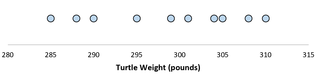
Для этой выборки из 10 черепах мы можем вычислить среднее значение выборки и стандартное отклонение выборки:

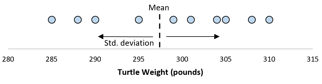
Предположим, что стандартное отклонение оказалось равным 8,68. Это дает нам представление о том, насколько распределен вес этих черепах.

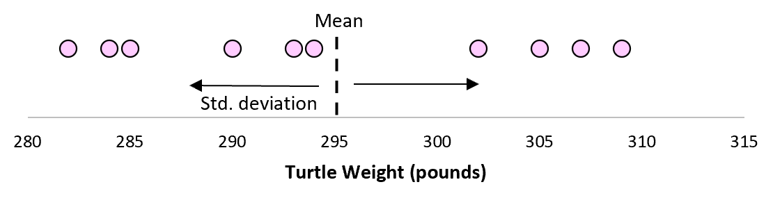
Но предположим, что мы собираем еще одну простую случайную выборку из 10 черепах и также проводим их измерения. Более чем вероятно, что эта выборка из 10 черепах будет иметь немного другое среднее значение и стандартное отклонение, даже если они взяты из одной и той же популяции:

Теперь, если мы представим, что мы берем повторные выборки из одной и той же совокупности и записываем выборочное среднее и выборочное стандартное отклонение для каждой выборки:

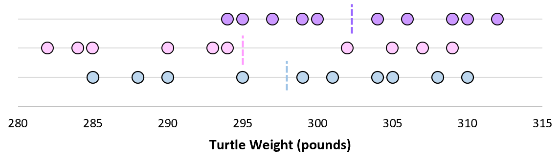
Теперь представьте, что мы наносим каждое среднее значение выборки на одну и ту же строку:

Стандартное отклонение этих средних значений известно как стандартная ошибка.

Формула для фактического расчета стандартной ошибки:

Стандартная ошибка = s/ √n

куда:

s: стандартное отклонение выборки
n: размер выборки

Какой смысл использовать стандартную ошибку?

Когда мы вычисляем среднее значение данной выборки, нас на самом деле интересует не среднее значение этой конкретной выборки, а скорее среднее значение большей совокупности, из которой взята выборка.

Однако мы используем выборки, потому что для них гораздо проще собирать данные, чем для всего населения. И, конечно же, среднее значение выборки будет варьироваться от выборки к выборке, поэтому мы используем стандартную ошибку среднего значения как способ измерить, насколько точна наша оценка среднего значения.

Вы заметите из формулы для расчета стандартной ошибки, что по мере увеличения размера выборки (n) стандартная ошибка уменьшается:

Стандартная ошибка = s/ √n

Это должно иметь смысл, поскольку большие размеры выборки уменьшают изменчивость и увеличивают вероятность того, что среднее значение нашей выборки ближе к фактическому среднему значению генеральной совокупности.

Когда использовать стандартное отклонение против стандартной ошибки

Если мы просто заинтересованы в измерении того, насколько разбросаны значения в наборе данных, мы можем использовать стандартное отклонение .

Однако, если мы заинтересованы в количественной оценке неопределенности оценки среднего значения, мы можем использовать стандартную ошибку среднего значения .

В зависимости от вашего конкретного сценария и того, чего вы пытаетесь достичь, вы можете использовать либо стандартное отклонение, либо стандартную ошибку.

Источник

Среднее арифметическое, как известно, используется для получения обобщающей характеристики некоторого набора данных. Если данные более-менее однородны и в них нет аномальных наблюдений (выбросов), то среднее хорошо обобщает данные, сведя к минимуму влияние случайных факторов (они взаимопогашаются при сложении).

Когда анализируемые данные представляют собой выборку (которая состоит из случайных значений), то среднее арифметическое часто (но не всегда) выступает в роли приближенной оценки математического ожидания. Почему приближенной? Потому что среднее арифметическое – это величина, которая зависит от набора случайных чисел, и, следовательно, сама является случайной величиной. При повторных экспериментах (даже в одних и тех же условиях) средние будут отличаться друг от друга.

Для того, чтобы на основе статистического анализа данных делать корректные выводы, необходимо оценить возможный разброс полученного результата. Для этого рассчитываются различные показатели вариации. Но то исходные данные. И как мы только что установили, среднее арифметическое также обладает разбросом, который необходимо оценить и учитывать в дальнейшем (в выводах, в выборе метода анализа и т.д.).

Интуитивно понятно, что разброс средней должен быть как-то связан с разбросом исходных данных. Основной характеристикой разброса средней выступает та же дисперсия.

Дисперсия выборочных данных – это средний квадрат отклонения от средней, и рассчитать ее по исходным данным не составляет труда, например, в Excel предусмотрены специальные функции. Однако, как же рассчитать дисперсию средней, если в распоряжении есть только одна выборка и одно среднее арифметическое?

Расчет дисперсии и стандартной ошибки средней арифметической

Чтобы получить дисперсию средней арифметической нет необходимости проводить множество экспериментов, достаточно иметь только одну выборку. Это легко доказать. Для начала вспомним, что средняя арифметическая (простая) рассчитывается по формуле:

где x_i – значения переменной,
n – количество значений.

Теперь учтем два свойства дисперсии, согласно которым, 1) — постоянный множитель можно вынести за знак дисперсии, возведя его в квадрат и 2) — дисперсия суммы независимых случайных величин равняется сумме соответствующих дисперсий. Предполагается, что каждое случайное значение x_i обладает одинаковым разбросом, поэтому несложно вывести формулу дисперсии средней арифметической:

Используя более привычные обозначения, формулу записывают как:

где σ² – это дисперсия, случайной величины, причем генеральная.

На практике же, генеральная дисперсия известна далеко не всегда, точнее совсем редко, поэтому в качестве оной используют выборочную дисперсию:

Стандартное отклонение средней арифметической называется стандартной ошибкой средней и рассчитывается, как квадратный корень из дисперсии.

Формула стандартной ошибки средней при использовании генеральной дисперсии

Формула стандартной ошибки средней при использовании выборочной дисперсии

Последняя формула на практике используется чаще всего, т.к. генеральная дисперсия обычно не известна. Чтобы не вводить новые обозначения, стандартную ошибку средней обычно записывают в виде соотношения стандартного отклонения выборки и корня объема выборки.

Назначение и свойство стандартной ошибки средней арифметической

Стандартная ошибка средней много, где используется. И очень полезно понимать ее свойства. Посмотрим еще раз на формулу стандартной ошибки средней:

Числитель – это стандартное отклонение выборки и здесь все понятно. Чем больше разброс данных, тем больше стандартная ошибка средней – прямо пропорциональная зависимость.

Посмотрим на знаменатель. Здесь находится квадратный корень из объема выборки. Соответственно, чем больше объем выборки, тем меньше стандартная ошибка средней. Для наглядности изобразим на одной диаграмме график нормально распределенной переменной со средней равной 10, сигмой – 3, и второй график – распределение средней арифметической этой же переменной, полученной по 16-ти наблюдениям (которое также будет нормальным).

Судя по формуле, разброс стандартной ошибки средней должен быть в 4 раза (корень из 16) меньше, чем разброс исходных данных, что и видно на рисунке выше. Чем больше наблюдений, тем меньше разброс средней.

Казалось бы, что для получения наиболее точной средней достаточно использовать максимально большую выборку и тогда стандартная ошибка средней будет стремиться к нулю, а сама средняя, соответственно, к математическому ожиданию. Однако квадратный корень объема выборки в знаменателе говорит о том, что связь между точностью выборочной средней и размером выборки не является линейной. Например, увеличение выборки с 20-ти до 50-ти наблюдений, то есть на 30 значений или в 2,5 раза, уменьшает стандартную ошибку средней только на 36%, а со 100-а до 130-ти наблюдений (на те же 30 значений), снижает разброс данных лишь на 12%.

Лучше всего изобразить эту мысль в виде графика зависимости стандартной ошибки средней от размера выборки. Пусть стандартное отклонение равно 10 (на форму графика это не влияет).

Видно, что примерно после 50-ти значений, уменьшение стандартной ошибки средней резко замедляется, после 100-а – наклон постепенно становится почти нулевым.

Таким образом, при достижении некоторого размера выборки ее дальнейшее увеличение уже почти не сказывается на точности средней. Этот факт имеет далеко идущие последствия. Например, при проведении выборочного обследования населения (опроса) чрезмерное увеличение выборки ведет к неоправданным затратам, т.к. точность почти не меняется. Именно поэтому количество опрошенных редко превышает 1,5 тысячи человек. Точность при таком размере выборки часто является достаточной, а дальнейшее увеличение выборки – нецелесообразным.

Подведем итог. Расчет дисперсии и стандартной ошибки средней имеет довольно простую формулу и обладает полезным свойством, связанным с тем, что относительно хорошая точность средней достигается уже при 100 наблюдениях (в этом случае стандартная ошибка средней становится в 10 раз меньше, чем стандартное отклонение выборки). Больше, конечно, лучше, но бесконечно увеличивать объем выборки не имеет практического смысла. Хотя, все зависит от поставленных задач и цены ошибки. В некоторых опросах участие принимают десятки тысяч людей.

Дисперсия и стандартная ошибка средней имеют большое практическое значение. Они используются в проверке гипотез и расчете доверительных интервалов.

Поделиться в социальных сетях:

Источник

Среднеквадратичная ошибка (Mean Squared Error) – Среднее арифметическое (Mean) квадратов разностей между предсказанными и реальными значениями Модели (Model) Машинного обучения (ML):

MSE как среднее дистанций между предсказаниями и реальными наблюдениями

Рассчитывается с помощью формулы, которая будет пояснена в примере ниже:

$$MSE = frac{1}{n} × sum_{i=1}^n (y_i — widetilde{y}_i)^2$$
$$MSEspace{}{–}space{Среднеквадратическая}space{ошибка,}$$
$$nspace{}{–}space{количество}space{наблюдений,}$$
$$y_ispace{}{–}space{фактическая}space{координата}space{наблюдения,}$$
$$widetilde{y}_ispace{}{–}space{предсказанная}space{координата}space{наблюдения,}$$

MSE практически никогда не равен нулю, и происходит это из-за элемента случайности в данных или неучитывания Оценочной функцией (Estimator) всех факторов, которые могли бы улучшить предсказательную способность.

Пример. Исследуем линейную регрессию, изображенную на графике выше, и установим величину среднеквадратической Ошибки (Error). Фактические координаты точек-Наблюдений (Observation) выглядят следующим образом:

Мы имеем дело с Линейной регрессией (Linear Regression), потому уравнение, предсказывающее положение записей, можно представить с помощью формулы:

$$y = M * x + b$$
$$yspace{–}space{значение}space{координаты}space{оси}space{y,}$$
$$Mspace{–}space{уклон}space{прямой}$$
$$xspace{–}space{значение}space{координаты}space{оси}space{x,}$$
$$bspace{–}space{смещение}space{прямой}space{относительно}space{начала}space{координат}$$

Параметры M и b уравнения нам, к счастью, известны в данном обучающем примере, и потому уравнение выглядит следующим образом:

$$y = 0,5252 * x + 17,306$$

Зная координаты реальных записей и уравнение линейной регрессии, мы можем восстановить полные координаты предсказанных наблюдений, обозначенных серыми точками на графике выше. Простой подстановкой значения координаты x в уравнение мы рассчитаем значение координаты ỹ:

Рассчитаем квадрат разницы между Y и Ỹ:

Сумма таких квадратов равна 4 445. Осталось только разделить это число на количество наблюдений (9):

$$MSE = frac{1}{9} × 4445 = 493$$

Само по себе число в такой ситуации становится показательным, когда Дата-сайентист (Data Scientist) предпринимает попытки улучшить предсказательную способность модели и сравнивает MSE каждой итерации, выбирая такое уравнение, что сгенерирует наименьшую погрешность в предсказаниях.

MSE и Scikit-learn

Среднеквадратическую ошибку можно вычислить с помощью SkLearn. Для начала импортируем функцию:

import sklearn
from sklearn.metrics import mean_squared_error

Инициализируем крошечные списки, содержащие реальные и предсказанные координаты y:

y_true = [5, 41, 70, 77, 134, 68, 138, 101, 131]
y_pred = [23, 35, 55, 90, 93, 103, 118, 121, 129]

Инициируем функцию mean_squared_error(), которая рассчитает MSE тем же способом, что и формула выше:

mean_squared_error(y_true, y_pred)

Интересно, что конечный результат на 3 отличается от расчетов с помощью Apple Numbers:

496.0

Ноутбук, не требующий дополнительной настройки на момент написания статьи, можно скачать здесь.

Автор оригинальной статьи: @mmoshikoo

Фото: @tobyelliott

Источник

Definition and basic properties[edit]

Predictor[edit]

Estimator[edit]

Proof of variance and bias relationship[edit]

In regression[edit]

Examples[edit]

Mean[edit]

Variance[edit]

Gaussian distribution[edit]

Interpretation[edit]

Applications[edit]

Loss function[edit]

Criticism[edit]

See also[edit]

Notes[edit]

References[edit]

Стандартное отклонение и стандартная ошибка: в чем разница?

Пример: стандартное отклонение против стандартной ошибки

Какой смысл использовать стандартную ошибку?

Когда использовать стандартное отклонение против стандартной ошибки

Расчет дисперсии и стандартной ошибки средней арифметической

Назначение и свойство стандартной ошибки средней арифметической

MSE и Scikit-learn