
Ограничение спектра
Если ограничить
спектр выше определенной частоты (fmв нашем примере), некоторые из проблем
могут быть решены. После этого можно
уверенно устанавливать частоту
дискретизацииfs= 2fmчто исключает элайсинг в восстанавливаемом
сигнале.
Ограничение спектра
производится с помощью фильтрации,
которая будет рассматриваться в лекции
3. Фильтрация гарантирует, что в
обрабатываемом сигнале не будет
высокочастотных составляющих, которые
могли бы привести к элайсингу.
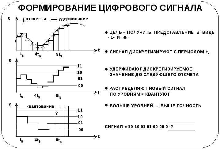
Формирование цифрового сигнала
Перед тем как ЦПОС
сможет обработать аналоговый сигнал,
его необходимо представить в цифровой
форме. Это единственный тип данных, с
которым может оперировать ЦПОС .
Формирование
цифрового сигнала, как правило, реализуется
в два этапа – дискретизации и квантования
(т. е. получения цифрового представления
отсчета). Этот процесс повторяется
периодически.
Дискретизация
Первый этап
формирования цифрового сигнала –
дискретизация. Из предыдущих рассуждений
известна безопасная частота дискретизации
сигнала. На практике дискретизируют
сигнал в соответствующий момент времени,
а затем удерживают полученное значение
отсчета до момента формирования
следующего отсчета. Отсчет сигнала
используют для получения его цифрового
представления.
Причина удерживания
величины отсчета может быть не совсем
очевидна. «Период удерживания» дает
время аналого-цифровому преобразователю
(АЦП) выполнить его преобразование.
Квантование
Для примера выбран
четырехуровневый 2-разрядный квантователь.
Квантователь определяет, куда попадает
значение конкретного отсчета в пределах
четырех уровней. Каждому уровню
присваивается 2-разрядный код в порядке
возрастания. На этом этапе полезно
напомнить, что
-
Двоичные
Десятичные
00
0
01
1
10
2
11
3
Определите последние
три уровня квантования на графике
Пауза
10 11 11
Точность
Количество уровней
квантования может быть любым, причем
чем оно больше, тем выше точность
цифрового представления. Мы рассмотрим
этот вопрос более внимательно позже.
Как и во всех технических задачах, в
данном случае должен быть найден
компромисс между точностью и стоимостью.
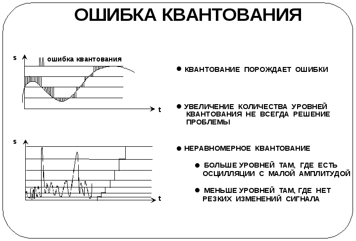
Ошибка квантования
Процесс квантования
сам по себе привносит ошибки. Существуют
два основных источника ошибок. Один из
них – дискретизация, в процессе которой
выбирают значение сигнала в дискретный
момент времени и затем удерживают его
до момента формирования следующего
отсчета. Второй источник ошибок возникает
как следствие работы квантователя.
Значение отсчета подтягивается либо
опускается до своего ближайшего
возможного цифрового представления
(т.е. уровня квантования). На графике,
соответствующем процедуре квантования,
показано семейство уровней ошибки,
имеющих место в данном случае.
Уменьшение ошибок квантования
Один из способов
уменьшения ошибок – увеличение количества
уровней квантования. Это, без сомнения,
в ряде случаев уменьшит ошибку, поскольку
любой отсчет будет располагаться ближе
к соседним уровням квантования, чем в
случае меньшего количества уровней.
Однако уменьшение
количества уровней квантования не
всегда является решением проблемы.
Рассмотрим случай, когда значения
сигнала сгруппированы в определенные
кластеры, как это показано на втором
графике. Нижняя часть графика соответствует
сильно осциллирующему сигналу с малыми
амплитудами, верхняя – слабо осциллирующему
с большими амплитудами. Если бы мы решили
использовать «неравномерное» квантование
сигнала данной формы, допуская больше
уровней квантования в диапазоне резких
изменений с малой амплитудой, мы смогли
бы более точно представить данный сигнал
в цифровой форме.
В большинстве
приложений квантователь имеет постоянный
размер шага, а входной сигнал
компрессируется. При восстановлении
выходной сигнал декомпрессируется.
Этот процесс называется «компандированием»
(от слов COMpressingиexPANDING).
Special Volume: Mathematical Modeling and Numerical Methods in Finance
Gilles Pagès, Jacques Printems, in Handbook of Numerical Analysis, 2009
Definition 3.1
A quantizer Γ ⊂ H is stationary (or self-consistent) if (there is a nearest-neighbor projection such that
XˆΓ = ProΓ (X) satisfying)
(3.3)XˆΓ=E(X|XˆΓ).
Note, in particular, that any stationary quantization satisfies EX = E
XˆΓ.
As shown by Proposition 3.1(c) any quadratic optimal quantizer at level N is stationary. Usually, at least when d ≥ 2, there are other stationary quantizers: indeed, the distortion function
DNX is |·|H-differentiable at N-quantizers x ∈ HN with pairwise distinct components and
∇DNX(x)=2(∫Ci(x)(xi-ξ)ℙX(dξ))1≤i≤N=2(E(XˆΓ(x)-X)1{XˆΓ(x)=xi})1≤i≤N.
Hence, any critical point of
DNX is a stationary quantizer.
Read full chapter
URL:
https://www.sciencedirect.com/science/article/pii/S157086590800015x
Digital Filters
Marcio G. Siqueira, Paulo S.R. Diniz, in The Electrical Engineering Handbook, 2005
2.11 Quantization in Digital Filters
Quantization errors in digital filters can be classified as:
- •
-
Round-off errors derived from internal signals that are quantized before or after more down additions;
- •
-
Deviations in the filter response due to finite word length representation of multiplier coefficients; and
- •
-
Errors due to representation of the input signal with a set of discrete levels.
A general, digital filter structure with quantizers before delay elements can be represented as in Figure 2.23, with the quantizers implementing rounding for the granular quantization and saturation arithmetic for the overflow nonlinearity.

FIGURE 2.23. Digital Filter Including Quantizers at the Delay Inputs
The criterion to choose a digital filter structure for a given application entails evaluating known structures with respect to the effects of finite word length arithmetic and choosing the most suitable one.
2.11.1 Coefficient Quantization
Approximations are known to generate digital filter coefficients with high accuracy. After coefficient quantization, the frequency response of the realized digital filter will deviate from the ideal response and eventually fail to meet the prescribed specifications. Because the sensitivity of the filter response to coefficient quantization varies with the structure, the development of low-sensitivity digital filter realizations has raised significant interest (Antoniou, 1993; Diniz et al., 2002).
A common procedure is to design the digital filter with infinite coefficient word length satisfying tighter specifications than required, to quantize the coefficients, and to check if the prescribed specifications are still met.
2.11.2 Quantization Noise
In fixed-point arithmetic, a number with a modulus less than one can be represented as follows:
(2.84)x=b0b1b2b3…bb,
where b0 is the sign bit and where b1b2b3 … bb represent the modulus using a binary code. For digital filtering, the most widely used binary code is the two’s complement representation, where for positive numbers b0 = 0 and for negative numbers b0 = 1. The fractionary part of the number, called x2 here, is represented as:
(2.85)x2={xif b0=0.2−|x|if b0=1.
The discussion here concentrates in the fixed-point implementation.
A finite word length multiplier can be modeled in terms of an ideal multiplier followed by a single noise source e(n) as shown in Figure 2.24.
FIGURE 2.24. Model for the Noise Generated after a Multiplication
For product quantization performed by rounding and for signal levels throughout the filter much larger than the quantization step q = 2−b, it can be shown that the power spectral density of the noise source ei(n) is given by:
(2.86)Pei(z)=q212=2−2b12.
In this case, ei(n) represents a zero mean white noise process. We can consider that in practice, ei(n) and ek(n + l) are statistically independent for any value of n or l (for i ≠ k). As a result, the contributions of different noise sources can be taken into consideration separately by using the principle of superposition.
The power spectral density of the output noise, in a fixed-point digital-filter implementation, is given by:
(2.87)Py(z)=σe2Σi=1KGi(z)Gi(z−1),
where Pei(ejw)=σe2, for all i, and each Gi(z) is a transfer function from multiplier output (gi(n)) to the output of the filter as shown in Figure 2.25. The word length, including sign, is b + 1 bits, and K is the number of multipliers of the filter.

FIGURE 2.25. Digital Filter Including Scaling and Noise Transfer Functions.
2.11.3 Overflow Limit Cycles
Overflow nonlinearities influence the most significant bits of the signal and cause severe distortion. An overflow can give rise to self-sustained, high-amplitude oscillations known as overflow limit cycles. Digital filters, which are free of zero-input limit cycles, are also free of overflow oscillations if the overflow nonlinearities are implemented with saturation arithmetic, that is, by replacing the number in overflow by a number with the same sign and with maximum magnitude that fits the available wordlength.
When there is an input signal applied to a digital filter, overflow might occur. As a result, input signal scaling is required to reduce the probability of overflow to an acceptable level. Ideally, signal scaling should be applied to ensure that the probability of overflow is the same at each internal node of the digital filter. This way, the signal-to-noise ratio is maximized in fixed-point implementations.
In two’s complement arithmetic, the addition of more than two numbers will be correct independently of the order in which they are added even if overflow occurs in a partial summation as long as the overall sum is within the available range to represent the numbers. As a result, a simplified scaling technique can be used where only the multiplier inputs require scaling. To perform scaling, a multiplier is used at the input of the filter section as illustrated in Figure 2.25.
It is possible to show that the signal at the multiplier input is given by:
(2.88)xi(n)=12πj∮cXi(z)zn−1dz=12π∫02πFi(ejω)X(ejω)ejωndω,
where c is the convergence region common to Fi(z) and X(z).
The constant λ is usually calculated by using Lp norm of the transfer function from the filter input to the multiplier input Fi(z), depending on the known properties of the input signal. The Lp norm of Fi(z) is defined as:
(2.89)‖Fi(ejω)‖p=[12π∫02π|Fi(ejω)|pdω]1p,
for each p ≥ 1, such that ∫02π|Fi(ejω)|pdω≤∞. In general, the following inequality is valid:
(2.90)|xi(n)| ≤ ‖Fi‖p‖X‖q, (1p+1q=1),
for p, q = 1, 2 and ∞.
The scaling guarantees that the magnitudes of multiplier inputs are bounded by a number Mmax when |x(n)| ≤ Mmax. Then, to ensure that all multiplier inputs are bounded by Mmax we must choose λ as follows:
(2.91)λ=1Max{‖F1‖p,…,‖F1‖p,…, ‖FK‖p},
which means that:
(2.92)‖F′i(ejω)‖p≤1, for‖X(ejω)‖q ≤ Mmax.
The K is the number of multipliers in the filter.
The norm p is usually chosen to be infinity or 2. The L∞ norm is used for input signals that have some dominating frequency component, whereas the L2 norm is more suitable for a random input signal. Scaling coefficients can be implemented by simple shift operations provided they satisfy the overflow constraints.
In case of modular realizations, such as cascade or parallel realizations of digital filters, optimum scaling is accomplished by applying one scaling multiplier per section.
As an illustration, we present the equation to compute the scaling factor for the cascade realization with direct-form second-order sections:
(2.93)λi=1‖∏j=1i−1Hj(z)Fi(z)‖p,
where:
Fi(z)=1z2+m1iz+m2i.
The noise power spectral density is computed as:
(2.94)Py(z)=σe2[3+3λ12∏i=1mHi(z)Hi(z−1)+5Σj=2m1λj2∏i=jmHi(z)Hi(z−1)],
whereas the output noise variance is given by:
(2.95)σo2=σe2[3+3λ12||∏i=1mHi(ejω)||22+5Σj=2m1λj2||∏i=jmHi(ejω)||22].
As a design rule, the pairing of poles and zeros is performed as explained here: poles closer to the unit circle pair with closer zeros to themselves, such that ||Hi(z)||p is minimized for p = 2 or p = ∞.
For ordering, we define the following:
(2.96)Pi=| |Hi(z)| |∞| |Hi(z)| |2.
For L2 scaling, we order the section such that Pi is decreasing. For L∞ scaling, Pi should be increasing.
2.11.4 Granularity Limit Cycles
The quantization noise signals become highly correlated from sample to sample and from source to source when signal levels in a digital filter become constant or very low, at least for short periods of time. This correlation can cause autonomous oscillations called granularity limit cycles.
In recursive digital filters implemented with rounding, magnitude truncation,72 and other types of quantization, limitcycles oscillations might occur.
In many applications, the presence of limit cycles can be harmful. Therefore, it is desirable to eliminate limit cycles or to keep their amplitude bounds low.
If magnitude truncation is used to quantize particular signals in some filter structures, it can be shown that it is possible to eliminate zero-input limit cycles. As a consequence, these digital filters are free of overflow limit cycles when overflow nonlinearities, such as saturation arithmetic, are used.
In general, the referred methodology can be applied to the following class of structures:
- •
-
State-space structures: Cascade and parallel realization of second-order state-space structures includes design constraints to control nonlinear oscillations (Diniz and Antoniou, 1986).
- •
-
Wave digital filters: These filters emulate doubly terminated lossless filters and have inherent stability under linear conditions as well as in the nonlinear case where the signals are subjected to quantization (Fettweis, 1986).
- •
-
Lattice realization: Modular structures allowing easy limit cycles elimination (Gray and Markel, 1975).
Read full chapter
URL:
https://www.sciencedirect.com/science/article/pii/B9780121709600500621
Special Volume: Mathematical Modeling and Numerical Methods in Finance
Huyên Pham, … Wolfgang J. Runggaldier, in Handbook of Numerical Analysis, 2009
4.2 Error analysis and rate of convergence
We state an error estimation between the optimal cost function Jopt and the approximated cost function
Jˆquant, in terms of
- •
-
the quantization errors Δk = ||Wk —
Wˆk||2 for the pair
Wk=(Πk,Yk), k = 0, …, n - •
-
the spatial step v and the grid size R for
Vkα, k = 0, …, n.
Theorem 4.1
Under H1, H2, H3, and H4, we have for all v0 ɛ ΓV
(4.5)|Jopt(υ0)-Jˆquant(υ0)|≤C1(n)Σk=0nΣj=0kΨk(v+C2R+Δk-j),
where
C1(n)=m+d+1[2(nL¯gf¯+M¯+3L¯gh¯)v(2L¯g)n2L¯g-1+f¯+h¯],
f¯=max ([ f ]sup,[ f ]Lip),
h¯=max([ h ]sup,[ h ]Lip),
L¯g=max ( L g,1),
M¯=max ( [ H ] Lip,1), C2 is the maximum value of H over
ΓV×A×∪kΓk×∪kΓk and ψ = (2d + 1)[H]Lip.
Proof
See Appendix B.
4.2.1 Convergence of the approximation
As a consequence of Zador’s theorem (see Graf and Luschgy [2000]), which gives the asymptotic behavior of the optimal quantization error, when the number of grid points goes to infinity, we can derive the following estimation on the optimal quantization error for the pair filter observation (see Pham, Runggaldier and Sellami [2004]):
limsupNk→∞Nk2m-1+dmin|Γk|≤Nk||Wk-Wˆk||22 ≤Ck(m,d),
where Ck(m, d) is a constant depending on m, d, and the marginal density of Yk. Therefore, the estimation (4.5) provides a rate of convergence for the approximation of Jopt of order
n2ΨnC1(n)(v+1R+1N1m-1+d),
when Nk = N is the number of points at each grid Γk used for the optimal quantization of Wk = (Πk, Yk), k = 1, …, n. We then get the convergence of the approximated cost function
Jˆquant to the optimal cost function Jopt when v goes to zero and N and R go to infinity. Moreover, by extending the approximate control
αˆk, k = 0, …, n − 1, to the continuous state space Km × ℝd × ℝ by
αˆk(π,y,υ)=αˆk(ProjΓk(π,y),ProjΓV(υ)), ∀(π,y,υ)∈K|m×ℝd×ℝ,
and by setting (by abuse of notation)
αˆk=αˆk(Πk,Yk,Vˆkαˆ) we get an approximate control
αˆ=(αˆk)k in A, which is ɛ-optimal for the original control problem (see Runggaldier [1991]) in the sense that for all ɛ > 0
J(υ0,αˆ)≤Jopt(υ0)+ɛ,
whenever N and R are large enough and v is small enough.
Read full chapter
URL:
https://www.sciencedirect.com/science/article/pii/S1570865908000094
Sampling Theory
Luis Chaparro, in Signals and Systems Using MATLAB (Second Edition), 2015
8.3.2 Quantization and Coding
Amplitude discretization of the sampled signal xs(t) is accomplished by a quantizer consisting of a number of fixed amplitude levels against which the sample amplitudes {x(nTs)} are compared. The output of the quantizer is one of the fixed amplitude levels that best represents {x(nTs)} according to some approximation scheme. The quantizer is a non-linear system.
Independent of how many levels or, equivalently, of how many bits are allocated to represent each level of the quantizer, in general there is a possible error in the representation of each sample. This is called the quantization error. To illustrate this, consider the 2-bit or four-level quantizer shown in Figure 8.12. The input of the quantizer are the samples {x(nTs)}, which are compared with the values in the bins [-2Δ,-Δ],[-Δ,0],[0,Δ], and [Δ,2Δ]. Depending on which of these bins the sample falls in it is replaced by the corresponding levels -2Δ,-Δ,0, or Δ, respectively. The value of the quantization step Δ for the four-level quantizer is
Figure 8.12. Four-level quantizer and coder.
(8.23)Δ=dynamic range of signal2b=2max|x(t)|22
where b = 2 is number of bits of the code assigned to each level. The bits assigned to each of the levels uniquely represents the different levels [-2Δ,-Δ,0,Δ]. As to how to approximate the given sample to one of these levels, it can be done by rounding or by truncating. The quantizer shown in Figure 8.12 approximates by truncation, i.e., if the sample kΔ≤x(nTs)<(k+1)Δ, for k = −2, −1,0,1, then it is approximated by the level kΔ.
To see how quantization and coding are done, and how to obtain the quantization error, let the sampled signal be
x(nTs)=x(t)|t=nTS
The given four-level quantizer is such that if the sample x(nTs) is such that
(8.24)kΔ≤x(nTs)<(k+1)Δ⇒xˆ(nTs)=kΔk=-2,-1,0,1
The sampled signal x(nTs) is the input of the quantizer and the quantized signal xˆ(nTs) is its output. So that whenever
-2Δ≤x(nTs)<-Δ⇒xˆ(nTs)=-2Δ-Δ≤x(nTs)<0⇒xˆ(nTs)=-Δ0≤x(nTs)<Δ⇒xˆ(nTs)=0Δ≤x(nTs)<2Δ⇒xˆ(nTs)=Δ
To transform the quantized values into unique binary 2-bit values, one could use a code such as
xˆ(nTs)⇒binary code-2Δ10-Δ110Δ00Δ01
which assigns a unique 2 bit binary number to each of the 4 quantization levels. Notice that the first bit of this code can be considered a sign bit, “1” for negative levels and “0” for positive levels.
If we define the quantization error as
ε(nTs)=x(nTs)-xˆ(nTs)
and use the characterization of the quantizer given by Equation (8.24) as
xˆ(nTs)≤x(nTs)≤xˆ(nTs)+Δ
by subtracting xˆ(nTs) from each of the terms gives that the quantization error is bounded as follows
(8.25)0≤ε(nTs)≤Δ
i.e., the quantization error for the four-level quantizer being considered is between 0 and Δ. This expression for the quantization error indicates that one way to decrease the quantization error is to make the quantization step Δsmaller. Increasing the number of bits of the A/D converter makes Δ smaller (see Equation (8.23) where the denominator is 2 raised to the number of bits) which in turn makes smaller the quantization error, and improves the quality of the A/D converter.
In practice, the quantization error is random and so it needs to be characterized probabilistically. This characterization becomes meaningful when the number of bits is large, and when the input signal is not a deterministic signal. Otherwise, the error is predictable and thus not random. Comparing the energy of the input signal to the energy of the error, by means of the so-called signal to noise ratio (SNR), it is possible to determine the number of bits that are needed in a quantizer to get a reasonable quantization error.
Example 8.5
Suppose we are trying to decide between an 8 and a 9 bit A/D converter for a certain application where the signals in this application are known to have frequencies that do not exceed 5 kHz. The dynamic range of the signals is 10 volts, so that the signal is bounded as −5 ≤ x(t) ≤ 5. Determine an appropriate sampling period and compare the percentage of error for the two A/Ds of interest.
Solution
The first consideration in choosing the A/D converter is the sampling period, so we need to get an A/D converter capable of sampling at fs = 1/Ts > 2 fmax samples/second. Choosing fs = 4 fmax = 20 k samples/second then Ts = 1/20 msec/sample or 50 microseconds/sample. Suppose then we look at the 8-bit A/D converter, the quantizer has 28 = 256 levels so that the quantization step is Δ=10/256 volts and if we use a truncation quantizer the quantization error would be
0≤ε(nTs)≤10/256
If we find that objectionable we can then consider the 9-bit A/D converter, with a quantizer of 29 = 512 levels and the quantization step Δ=10/512 or half that of the 8-bit A/D converter, and
0≤ε(nTs)≤10/512
So that by increasing one bit we cut the quantization error in half from the previous quantizer. Inputting a signal of constant amplitude 5 into the 9-bit A/D gives a quantization error of [(10/512)/5] × 100% = (100/256)% ≈ 0.4% in representing the input signal. For the 8-bit A/D it would correspond to 0.8% error. ▪
Read full chapter
URL:
https://www.sciencedirect.com/science/article/pii/B9780123948120000085
Compression
StéphaneMallat , in A Wavelet Tour of Signal Processing (Third Edition), 2009
Weighted Quantization and Regions of Interest
Visual distortions introduced by quantization errors of wavelet coefficients depend on the scale 2j. Errors at large scales are more visible than at fine scales [481]. This can be taken into account by quantizing the wavelet coefficients with intervals Δj=Δwj that depend on the scale 2j. For R¯≤1 bit/pixel, wj = 2−j is appropriate for the three finest scales. The distortion in (10.34) shows that choosing such weights is equivalent to minimizing a weighted mean-square error.
Such a weighted quantization is implemented like in (10.35) by quantizing weighted wavelet coefficients fB[m]/wj with a uniform quantizer. The weights are inverted during the decoding process. JPEG-2000 supports a general weighting scheme that codes weighted coefficients w[m]fB[m] where w[m] can be designed to emphasize some region of interest Ω ⊂ [0, 1]2 in the image. The weights are set to w[m] = w > 1 for the wavelet coefficients fB[m]=〈f,ψj,p,q1〉 where the support of ψj,p,q1 intersects Ω. As a result, the wavelet coefficients inside Ω are given a higher priority during the coding stage, and the region Ω is coded first within the compressed stream. This provides a mechanism to more precisely code regions of interest in images—for example, a face in a crowd.
Read full chapter
URL:
https://www.sciencedirect.com/science/article/pii/B9780123743701000148
Signal and Image Representation in Combined Spaces
Zoran. Cvetković, Martin. Vetterli, in Wavelet Analysis and Its Applications, 1998
6.1 Two lemmas on frames of complex exponentials
Estimates of bounds on the quantization error in Subsection 4.3 are derived from the next two lemmas [5].
Lemma 1
Letejλnωbe a frame in L2[− σ, σ]. If M is any constant and {μn} is a sequence satisfying |μn − λn| ≤ M, for all n, then there is a number C = C(M, σ, {λn}) such that
(6.1.1)∑n|fμn|2∑n|fλn|2≤C
for every cr-bandlimited signal f(x).
Lemma 2
Letejλnωbe a frame in L2[− σ, σ], with bounds 0 < A ≤ B < ∞ and δ a given positive number. If a sequence { μn } satisfies | λn − μn < δ for all n, then for every σ-bandlimited signal f(x)
(6.1.2)A1−C2||f||2≤∑n|fμn|2≤B(1+C)2||f||2,
where
(6.1.3)C=BAeγδ−12
Remark 1
If δ in the statement of Lemma 2 is chosen small enough, so that C is less then 1, then ejμnω is also a frame in L2[− σ, σ]. Moreover, there exists some δ 1/4 ({λn},σ), such that whenever δ < δ 1/4 ({λn }, σ), ejμnω is a frame with frame bounds A/A and 9B/4.
Read full chapter
URL:
https://www.sciencedirect.com/science/article/pii/S1874608X98800125
Converting analog to digital signals and vice versa
Edmund Lai PhD, BEng, in Practical Digital Signal Processing, 2003
2.3.3 Non-uniform quantization
One of the assumptions we have made in analyzing the quantization error is that the sampled signal amplitude is uniformly distributed over the full-scale range. This assumption may not hold for certain applications. For instance, speech signals are known to have a wide dynamic range. Voiced speech (e.g. vowel sounds) may have amplitudes that span the entire full-scale range, while softer unvoiced speech (e.g. consonants such as fricatives) usually have much smaller amplitudes. In addition, an average person only speaks 60% of the time while she/he is talking. The remaining 40% are silence with negligible signal amplitude.
If uniform quantization is used, the louder voiced sounds will be adequately represented. However, the softer sounds will probably occupy only a small number of quantization levels with similar binary values. This means that we would not be able to distinguish between the softer sounds. As a result, the reconstructed analog speech from these digital samples will not nearly be as intelligible as the original.
To get around this problem, non-uniform quantization can be used. More quantization levels are assigned to the lower amplitudes while the higher amplitudes will have less number of levels. This quantization scheme is shown in Figure 2.17.

Figure 2.17. Non-uniform quantization
Alternatively, a uniform quantizer can still be used, but the input signal is first compressed by a system with an input–output relationship (or transfer function) similar to that shown in Figure 2.18.

Figure 2.17. Non-uniform quantization
Alternatively, a uniform quantizer can still be used, but the input signal is first compressed by a system with an input–output relationship (or transfer function) similar to that shown in Figure 2.18.
Figure 2.18. μ-law compression characteristics
The higher amplitudes of the input signal are compressed, effectively reducing the number of levels assigned to it. The lower amplitude signals are expanded (or non-uniformly amplified), effectively making it occupy a large number of quantization levels. After processing, an inverse operation is applied to the output signal (expanding it). The system that expands the signal has an input-output relationship that is the inverse of the compressor. The expander expands the high amplitudes and compresses the low amplitudes. The whole process is called companding (COMpressing and exPANDING).
Companding is widely used in public telephone systems. There are two distinct companding schemes. In Europe, A-law companding is used and in the United States, μ-law companding is used.
μ-law compression characteristic is given by the formula:
y=ymaxln[1+μ(|x|xmax)]ln(1+μ)sgn(x)
where
Here, x and y represent the input and output values, and xmax and ymax are the maximum positive excursions of the input and output, respectively. μ is a positive constant. The North American standard specifies μ to be 255. Notice that μ = 0 corresponds to a linear input-output relationship (i.e. uniform quantization). The compression characteristic is shown in Figure 2.18.
The A-law compression characteristic is given by
y={ymaxA(|x|xmax)1+lnAsgn(x),x<|x|xmax≤1Aymax1+ln[A(|x|xmax)]1+lnAsgn(x),1A<|x|xmax<1
Here, A is a positive constant. The European standard specifies A to be 87.6. Figure 2.19 shows the characteristic graphically.

Figure 2.19. The A-law compression characteristics
Read full chapter
URL:
https://www.sciencedirect.com/science/article/pii/B9780750657983500023
A to D and D to A conversions
A.C. Fischer-Cripps, in Newnes Interfacing Companion, 2002
2.5.3 Resolution and quantisation noise
Now, a very interesting problem arises when analog data is to be stored in a digital system like a computer. The problem is that the data can only be represented by the range of numbers allowed for by the analog to digital converter. For example, for an 8-bit ADC, then the magnitude of the full range of the original analog data would have to be distributed between the binary numbers 00000000 to 11111111, or 0 to 255 in decimal. Numbers that don’t fit exactly with an 8-bit integer have to be rounded up or down to the nearest one and then stored.
If the ADC were able to accept input voltages from 0 to 5 volts, then full scale, or 5 volts, on the input would correspond to the number 255 on the output. The resolution of the ADC would be:
5255=0.0196V
Thus, for an input range of 0 to 5 volts, in this example, the resolution of the ADC would be 19.6 mV per bit or 0.39%. A 12-bit ADC would have a resolution of 1.22 mV per bit (0.02%) since it may divide the 5 volts into 4095 steps rather than 255.
In general, the resolution of an N bit ADC is:
Δ=Vref2N
where Vref is the range of input for the ADC in volts.
Quantisation noise
The quantisation error Δe is ± half a bit (LSB) and describes the inherent fundamental error associated with the process of dividing a continuous analog signal into a finite number of bits.
Δe=Vref2(2N)
The quantisation error is random, in that rounding up or down of the signal will occur with equal probability. This randomness leads to the digital signal containing quantisation noise, of a fixed amplitude, and a uniform spread of frequencies. The rms value in volts of the quantisation noise signal is given by:
The quantization noise level places a limit on the signal to noise ratio achievable with a particular ADC.
Read full chapter
URL:
https://www.sciencedirect.com/science/article/pii/B9780750657204501121
From Array Theory to Shared Aperture Arrays
NICHOLAS FOURIKIS, in Advanced Array Systems, Applications and RF Technologies, 2000
2.5.6.2 Amplitude, Phase, and Delay Quantization Errors
In this section we shall consider the impact of amplitude, phase, and delay quantization errors on the array radiation pattern. Our treatment will be brief, however, because these topics have been explored in some detail in many references, including the book [150].
Amplitude quantization (AQ) lobes occur because the amplitude control of the array illumination is implemented at the subarray level rather than at the antenna element level. By analogy with conventional array theory, grating lobes for an array having rectangular subarray lattices will occur in sine space at locations given by [136]
(2.84)uQ=u0±p λsx vq=v0±q λsy p, q=1, 2, …
where sx and sy are the inter-subarray spacing in the x and y directions rather than the interelement spacing more typically associated with these equations. As can be seen the positions of the AQ lobes can be altered by varying the number of subarray elements, a procedure that changes sx and sy.
If we restrict attention to subarrays, of length L, formed along the x-direction, the nulls of the radiation pattern corresponding to the subarray, are at angular distances ±p (λ/L); for contiguous subarrays L = sx so the positions of the nulls coincide with the positions of the grating lobes. When all subarrays are uniformly illuminated, the grating lobes have negligible power levels. However when the subarray illumination has a suitable taper to lower the array sidelobes, the main beam and grating lobes are broadened so that the resulting array radiation pattern has split grating lobes resembling the monopulse radiation patterns. This is clearly seen in the grating lobes of the array radiation pattern illustrated in Figure 2.19b.
If the array has m subarrays of n elements, then the peak power of the AQ lobes, Gp, is given by [151]
(2.85)Gp=m2n2sin2(πp/n)
where p = ±1, ±2, ±3, … and B0 is the beam broadening factor or the ratio of HPBWs of the broadened beam corresponding to a uniformly illuminated array. For certain applications the AQ lobes can be objectionable, even at the −40 dB level, if the lobes enter the visible space at some scanning angle.
Modern phased arrays utilize digital phase-shifters to direct the beam anywhere within the array surveillance volume. The inserted phases are therefore only approximations of the required phases.
If an N-bit phase-shifter is used, the least significant phase, ϕ0, is given by the equation
(2.86)ϕ0=2π2N
These quantization errors give rise to array grating lobes resembling those due to AQ but without the characteristic monopulse feature. Let u0 and us be the direction cosines of the intended and actual directions the array is pointed. The worst case occurs when the error build-up and its correction are entirely periodic, in which case the array is divided into virtual subarrays and each subarray has the same phase error gradient. This occurs when the distance between subarray centers is given by [151]
(2.87)|MΔϕ−MΔϕs|=2πsλM|u0−us|=2π2N
where M is the number of antenna elements in the virtual subarray and s is the interelement spacing. If u0–us is known, M can be derived from equation (2.87). The virtual subarraying induces grating lobes to form, and the power in each lobe is given by [151]
(2.88)PGL|p=[π2N1Msin(p′π/M)]2
where p′ = p + (1/2N) and p = ±1, ±2, ±3,… In Table 2.13 we have tabulated the power in the first grating lobe as a function of M and N; as can be seen, PGL|p can reach a high level of approximately −14 dB, when M = 2 and N = 3. As the number of bits used increases, the first grating lobe power decreases dramatically. The power in the second grating lobe is even lower.
Table 2.13. The first grating lobe power (in –dB) of an array as function of N and M
| M | |||||
|---|---|---|---|---|---|
| N | 2 | 4 | 6 | 8 | 10 |
| 3 | 13.97 | 17.92 | 18.57 | 18.80 | 18.90 |
| 4 | 20.11 | 23.57 | 24.15 | 24.35 | 24.45 |
| 5 | 26.17 | 29.39 | 29.94 | 30.13 | 30.44 |
| 6 | 32.20 | 35.31 | 35.84 | 36.03 | 36.11 |
It is often economical to steer the beam of a large array such as the COBRA DANE [118], operating over a small fractional bandwidth, by the use of time delays inserted at the subarray level, and phase-shifters at the array element. The resulting grating lobe power PD due to delay quantization is given by [151]
(2.89)PD|GP=π2X2sin2π[X+p/M]
where
X=μ0sλ0Δff0
If the array fractional bandwidth Δflf0 is much less than 0.1, the power in the grating lobes is negligible.
The COBRA DANE system has a 95 ft (30 m) aperture that is divided into 96 subarrays each having 160 antenna elements. If the array is pointed 22° in elevation off the aperture boresight, the top subarray receives a 36 ns time delay with respect to the bottom subarray. With this arrangement the incoming power is collimated over a bandwidth of 200 MHz [118].
Read full chapter
URL:
https://www.sciencedirect.com/science/article/pii/B9780122629426500044
Digital filter realizations
Edmund Lai PhD, BEng, in Practical Digital Signal Processing, 2003
8.7 Finite word-length effects
The number of bits that is used to represent numbers, called word-length, is often dictated by the architecture of DSP processor. If specialized VLSI hardware is designed, then we have more control over the word-length. In both cases we need to tradeoff the accuracy with the computational complexity. No matter how many bits are available for number representation, it will never be enough for all situations and some rounding and truncation will still be required.
For FIR digital filters, the finite word-length affects the results in the following ways:
- •
-
Coefficient quantization errors.
The coefficient we arrived at in the approximation stage of filter design assumes that we have infinite precision. In practice, however, we have the same word-length limitations on the coefficients as that on the signal samples. The accuracy of filter coefficients will affect the frequency response of the implemented filter.
- •
-
Round-off or truncation errors resulting from arithmetic operations.
Arithmetic operations such as addition and multiplication often give results that require more bits than the word-length. Thus truncation or rounding of the result is needed. Some filter structures are more sensitive to these errors than others.
- •
-
Arithmetic overflow.
This happens when some intermediate results exceed the range of numbers that can be represented by the given word-length. It can be avoided by careful design of the algorithm scale.
For IIR filters, our analysis of finite word-length effects will need to include one more factor: product round-off errors. The round-off or truncation errors of the output sample at one time instant will affect the error of the next output sample because of the recursive nature of the IIR filters. Sometimes limit cycles can occur.
We shall look at these word-length effects in more detail.
8.7.1 Coefficient quantization errors
Let us consider the low-pass FIR filter that has been designed by using Kaiser windows in section 6.4.4. The coefficients obtained are listed in Table 8.1. The table also shows the values of the coefficients if they are being quantized into 8 bits. The magnitude responses of the filter, both before and after coefficient quantization, are shown in Figure 8.20.
Table 8.1.
| N | Coefficient |
|---|---|
| 0 | −0.0016 |
| 1, 21 | 0.0022 |
| 2, 10 | 0.0026 |
| 3, 19 | −0.0117 |
| 4, 18 | 0.1270 |
| 5, 17 | 0.0071 |
| 6, 16 | −0.0394 |
| 7, 15 | −0.0466 |
| 8, 14 | 0.0117 |
| 9, 13 | −0.1349 |
| 10, 12 | 0.2642 |
| 11 | 0.6803 |

Figure 8.20. Magnitude response of a low-pass FIR filter before and after coefficient quantization
The quantized filter has violated the specification of the stopband. Clearly in this case, more than 8 bits are required for the filter coefficients.
The minimum number of bits needed for the filter coefficients can be found by computing the frequency response of the coefficient-quantized filter. A trial-and-error approach can be used. However, it will be useful to have some guideline for estimating the word-length requirements of a specific filter.
The quantized coefficients and the unquantized ones are related by
hq(n)=h(n)+e(n),n=0,1,…,N−1
and shown in Figure 8.21.
Figure 8.21. Model of coefficient quantization
This relationship can also be established in the frequency domain as in Figure 8.22.

Figure 8.22. Frequency domain model of coefficient quantization
Here H(ω) is the frequency response of the original filter and E(ω) is the error in the frequency response due to coefficient quantization.
If the direct form structure is used, assuming rounding, the following bounds for the magnitude of the error spectrum are most commonly used:
|E(ω)|=N2−B|E(ω)|=2−B(N/3)1/2|E(ω)|=2−B[13(NlnN)1/2]
where B is the number of bits used for representing the filter coefficients. The first bound is a worst case absolute bound and is usually over pessimistic. The other two are based on the assumption that the error e(n) is uniformly distributed with zero mean. They generally provide better estimates for the word-length required.
Example 8.6
For the low-pass filter designed in section 6.4.4, we have shown that 8-bit word-length is not sufficient for the coefficients. The order of the filter is N = 22. The stopband attenuation is specified to be at least 50 dB down.
So we need at least 10 bits for the coefficients. The resulting magnitude response is shown in Figure 8.23.
Figure 8.23. Coefficient quantized filter response
For IIR filters, the coefficient quantization error may have one more effect: instability. The stability of a filter depends on the location of the roots of the denominator polynomial in the transfer function. Consider a second order section of an IIR filter (since it is the basic building block of higher order filters) with transfer function
H(z)=b0+b1z−1+b2z−11+a1z−1+a2z−1
The roots of the denominator polynomial, or poles of the transfer function, are located at
p1=12[−a1+a12−4a2]p2=12[−a1−a12−4a2]
They may either be complex conjugate pairs or are both real. If they are complex conjugate pairs, they can be represented as having a magnitude and an angle:
where
For stability, the magnitude of these poles must be less than 1. This applies to both real and complex poles. So the test for stability for the second coefficient is
From the above equation for the angle, the arguments to the arc-cosine function must have a magnitude that is less than or equal to 1. So the test for stability for the first coefficient is
Both these tests must be satisfied at the same time for the IIR filter to remain stable.
8.7.2 Rounding and truncation
It is inevitable that some numbers are being represented by less number of bits than what is required to represent them exactly. For instance, when we multiply two n-bit numbers we have a result that is at most 2n-bits long. This result will still have to be represented using n-bits. Thus rounding or truncation will be needed. The characteristics of the errors introduced depend on how the numbers are represented.
Consider the n-bit fixed point representation of a number x, which requires nu bits to represent exactly, with n < nu. For positive numbers, both sign-magnitude and 2′s complement representations are identical. The error introduced by truncation is
with the largest error discarding all (nu−n) bits, (all being 1s).
For negative numbers represented using sign-magnitude format, truncation reduces the magnitude of the numbers and hence the truncation error is positive.
So the truncation error for sign-magnitude format is in the range
−(2−n−2−nu)≤Et≤(2−n−2−nu)
With 2′s complement representation, truncation of a negative number will increase the magnitude of the number and so the truncation error is negative.
So the truncation error for 2′s complement format is still in the range
Now consider round-off errors of the above fixed-point representations. In this case, the error is independent of the type of representation and it may either be positive or negative and is symmetrical about zero.
−12(2−n−2−nu)≤Et≤12(2−n−2−nu)
In floating point representations, the resolution is not uniform as discussed before. So the truncation and round-off errors are proportional to the number. It is more useful to consider the relative error defined as
where Q(x) is the number after truncation or rounding.
If the mantissa is represented by 2′s complement using n-bits, then the relative truncation errors has the bounds:
−2−n+1<et≤0,x>00≤et<2−n+1,x<0
The relative round-off error is in the range:
8.7.3 Overflow errors
Overflow occurs when two large numbers of the same sign are added and the result exceeds the word-length. If we use 2′s complement representation, as long as the final result is within the word-length, overflow of partial results is unimportant. If the final result does cause overflow, it may lead to serious errors in the system. Overflow can be avoided by detecting and correcting the error when it occurs. However, this is a rather expensive approach. A better way is to try and avoid it by scaling the data or the filter coefficients.
Consider an N-th order FIR filter. The output sample at time instant n is given by
Assume that the magnitudes of the input and the filter coefficients are less than 1. Then the magnitude of the output is
|y(n)|≤∑m=0N−1|h(m)||x(n−m)|
In the worst case,
A scaling factor G can be chosen as
The filter coefficients are all scaled by this factor
In this way, the maximum output magnitude of the filter will always be less than or equal to 1 and overflow is completely avoided.
However, this scaling method is very conservative. The worst case signal will hardly ever occur in practice. Two other less conservative scaling factors are usually chosen instead. The first one is defined by
G2=‖h‖2=[∑nh2(n)]1/2≤‖h‖1
This scaling improves the signal to quantization noise ratio. The trade-off is that there is a possibility of overflow. Another scaling factor, given by
guarantees that the steady-state response of the system to a sine wave will not overflow. This frequency domain-scaling factor is often the preferred method.
Scaling is even more important for IIR filters because an overflow in the current output sample affects many output samples following that one. In some cases, overflow can cause oscillation and seriously impair the usefulness of the filter. Only by resetting the filter can we recover from these oscillations.
The same set of scaling factors described above can be used for IIR filters. However, the frequency domain measure is more useful because the duration of the impulse response in this case is infinite. The procedure is illustrated by an example.
Example 8.7
An IIR filter is designed based on a 4th order elliptic low-pass filter. The filter transfer function is given by
H(z)=1+1.621784z−1+z−21−0.04030703z−1+0.2332662z−2·1+0.7158956z−1+z−21+0.0514214z−1+0.7972861z−2=H1(z)H2(z)
which is decomposed into a cascade of two second order sections.
The transpose structure of section 1 is shown in Figure 8.24.

Figure 8.24. Transpose structure of section 1
The impulse response and magnitude response of this section are as shown in Figure 8.25.

Figure 8.24. Transpose structure of section 1
The impulse response and magnitude response of this section are as shown in Figure 8.25.
Figure 8.25. The impulse and magnitude responses of section 1
Table 8.2 shows the three different scaling factors that can be used.
Table 8.2.
| Output | G1 | G2 | G3 |
|---|---|---|---|
| y1 | 5.30748 | 2.7843 | 4.38 |
| y11 | 1.7715 | 0.9774 | 1.28 |
| y12 | 4.30748 | 2.5985 | 3.67 |
Apart from the output of the section, the output of each internal adder within the section has to be examined as well. The impulse response at y11 and y12 and their frequency responses
H11(z)=Y11(z)X(z)=0.766733805−0.781377681z−11−0.40307027997z−1+0.766733805z−2H12(z)=Y12(z)X(z)=2.024854296+0.766733805z−11−0.4030702997z−1+0.2332661953z−2
are shown in Figures 8.26 and 8.27 respectively.

Figure 8.26. Frequency response H11(z)

Figure 8.26. Frequency response H11(z)
Figure 8.27. Frequency response H12(z)
Their corresponding scaling factors are also given in Table 8.2. Having decided on the particular type of scaling factor to be used, the largest one in that column should be chosen for scaling.
The same procedure can be followed to determine the scaling factor for the second section.
8.7.4 Limit cycles
Although we have been treating digital filters as linear systems, the fact is that a real digital filter is non-linear. This is due to quantization, round off, truncation, and overflow. A filter designed as a linear system, which is stable, may oscillate when an overflow occurs. This type of oscillation is called a limit cycle. Limit cycles due to round-off/truncation and overflow are illustrated by two examples.
Example 8.8
A first order IIR filter has the following different equation:
For α = 0.75, the output samples y(n) obtained using initial condition y(0) = 6 and a zero input x(n) = 0 for n ≥ 0 are listed in Table 8.3 and plotted in Figure 8.28(a). It shows that the output quickly decays to zero. If y(n) is rounded to the nearest integer, then after some time the output remains at 2. This is shown in Figure 8.28(b) and listed in Table 8.3.
Table 8.3.
| n | y(n), infinite precision | y(n), rounding |
|---|---|---|
| 0 | 6 | 6 |
| 1 | 4.5 | 5 |
| 2 | 3.38 | 4 |
| 3 | 2.53 | 3 |
| 4 | 1.90 | 2 |
| 5 | 1.42 | 2 |
| 6 | 1.07 | 2 |
| 7 | 0.80 | 2 |
| 8 | 0.60 | 2 |
| 9 | 0.45 | 2 |
| 10 | 0.3375 | 2 |

Figure 8.28. Output values before and after rounding
For α = −0.75, the output oscillates briefly and decays to zero for the infinite precision version. If the result is rounded to the nearest integer, then the output oscillates between −2 and +2. These signals are plotted in Figure 8.29 and listed in Table 8.4.
Figure 8.29. Output with and without rounding
Table 8.4.
| n | y(n), infinite precision | y(n), rounding |
|---|---|---|
| 0 | 6 | 6 |
| 1 | −4.5 | −5 |
| 2 | 3.38 | 4 |
| 3 | −2.53 | −3 |
| 4 | 1.90 | 2 |
| 5 | −1.42 | −2 |
| 6 | 1.07 | 2 |
| 7 | −0.80 | −2 |
| 8 | 0.60 | 2 |
| 9 | −0.45 | −2 |
| 10 | 0.3375 | 2 |
Example 8.9
A filter with transfer function
is stable filter. A 2′s complement overflow non-linearity is added to the filter structure as shown in Figure 8.30.

Figure 8.30. FIR filter structure with overflow non-linearity added
The transfer function of the non-linearity itself is shown in Figure 8.31.

Figure 8.30. FIR filter structure with overflow non-linearity added
The transfer function of the non-linearity itself is shown in Figure 8.31.
Figure 8.31. Transfer function of overflow non-linearity
According to the notations of Figure 8.30, if the input is zero,
x1(n+1)=x2(n)x2(n+1)=NL[−0.5×1(n)+x2(n)]
With an initial condition of
At the next time instant, we have
x1(n)=(−1)n0.8×2(n)=(−1)n+10.8
In fact, for n ≥ 1,
x1(1)=−0.8×2(1)=NL[−0.5×1(0)+x2(0)]=NL[−1.2]=+0.8
Thus the output oscillates between 0.8 and −0.8.
Note that the limit cycle will only start if there is a previous overflow. If no overflow occurs the system remains linear.
Read full chapter
URL:
https://www.sciencedirect.com/science/article/pii/B9780750657983500084
Дорогие читатели, меня зовут Феликс Арутюнян. Я студент, профессиональный скрипач. В этой статье хочу поделиться с Вами отрывком из моей презентации, которую я представил в университете музыки и театра Граца по предмету прикладная акустика.
Рассмотрим теоретические аспекты преобразования аналогового (аудио) сигнала в цифровой.
Статья не будет всеохватывающей, но в тексте будут гиперссылки для дальнейшего изучения темы.
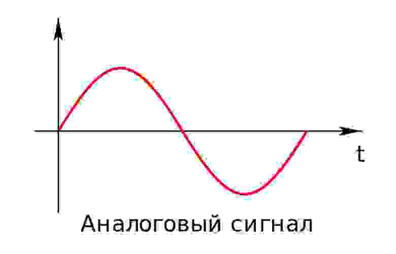
Чем отличается цифровой аудиосигнал от аналогового?
Аналоговый (или континуальный) сигнал описывается непрерывной функцией времени, т.е. имеет непрерывную линию с непрерывным множеством возможных значений (рис. 1).
рис. 1
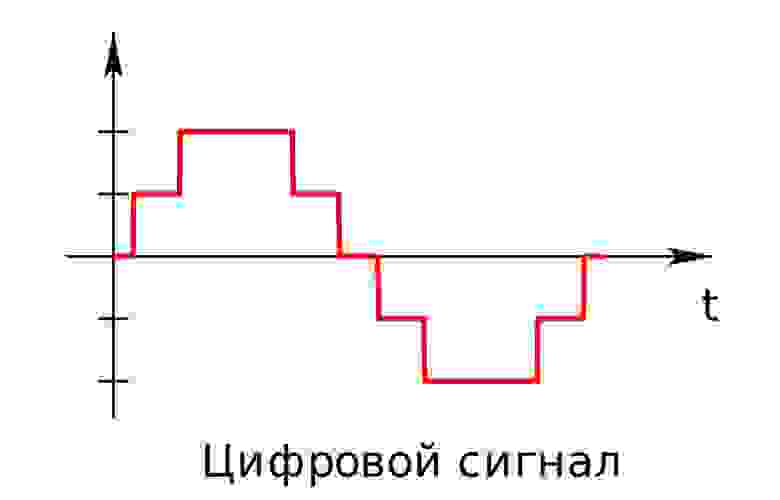
Цифровой сигнал — это сигнал, который можно представить как последовательность определенных цифровых значений. В любой момент времени он может принимать только одно определенное конечное значение (рис. 2).
рис. 2
Аналоговый сигнал в динамическом диапазоне может принимать любые значения. Аналоговый сигнал преобразуется в цифровой с помощью двух процессов — дискретизация и квантование. Очередь процессов не важна.
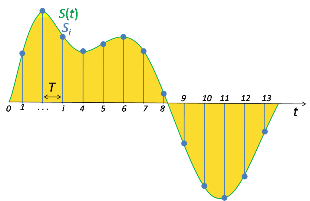
Дискретизацией называется процесс регистрации (измерения) значения сигнала через определенные промежутки (обычно равные) времени (рис. 3).
рис. 3
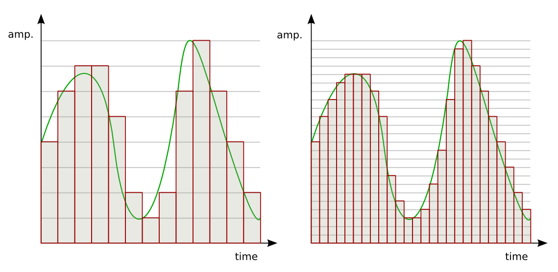
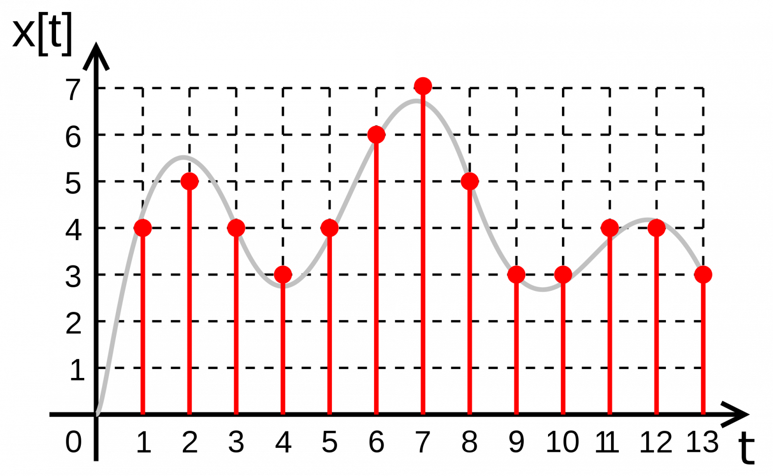
Квантование — это процесс разбиения диапазона амплитуды сигнала на определенное количество уровней и округление значений, измеренных во время дискретизации, до ближайшего уровня (рис. 4).
рис. 4
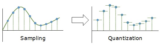
Дискретизация разбивает сигнал по временной составляющей (по вертикали, рис. 5, слева).
Квантование приводит сигнал к заданным значениям, то есть округляет сигнал до ближайших к нему уровней (по горизонтали, рис. 5, справа).
рис. 5
Эти два процесса создают как бы координатную систему, которая позволяет описывать аудиосигнал определенным значением в любой момент времени.
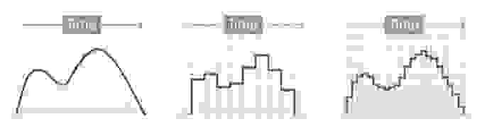
Цифровым называется сигнал, к которому применены дискретизация и квантование. Оцифровка происходит в аналого-цифровом преобразователе (АЦП). Чем больше число уровней квантования и чем выше частота дискретизации, тем точнее цифровой сигнал соответствует аналоговому (рис. 6).
рис. 6
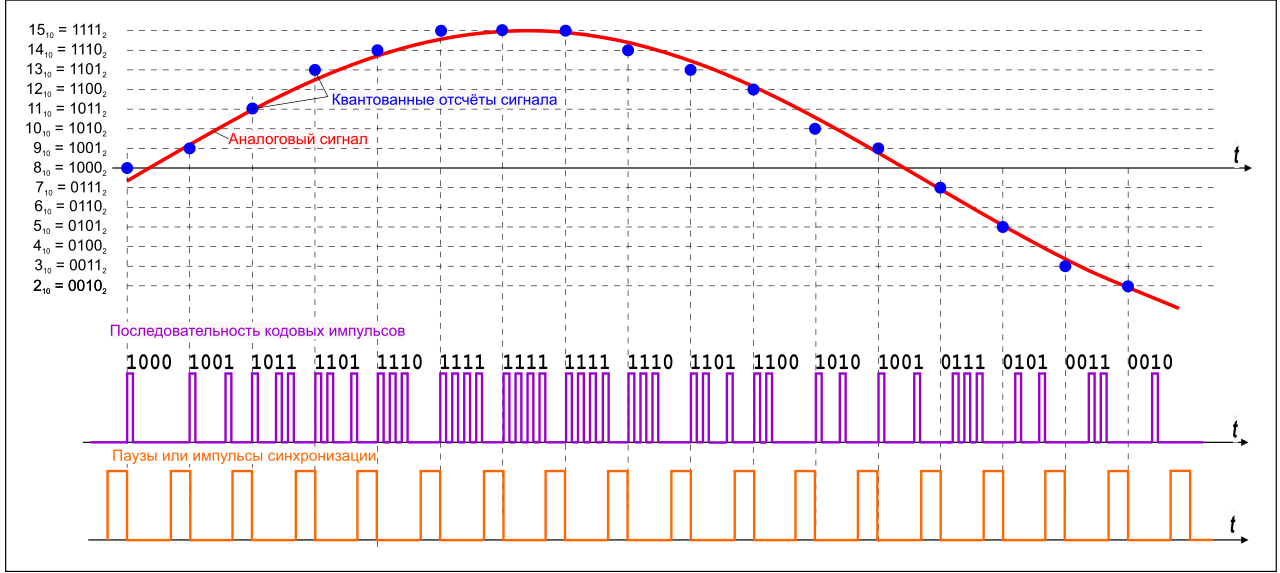
Уровни квантования нумеруются и каждому уровню присваивается двоичный код. (рис. 7)
рис. 7
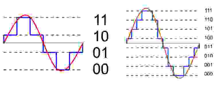
Количество битов, которые присваиваются каждому уровню квантования называют разрядностью или глубиной квантования (eng. bit depth). Чем выше разрядность, тем больше уровней можно представить двоичным кодом (рис. 8).
рис. 8.
Данная формула позволяет вычислить количество уровней квантования:
Если N — количество уровней квантования,
n — разрядность, то

Обычно используют разрядности в 8, 12, 16 и 24 бит. Несложно вычислить, что при n=24 количество уровней N = 16,777,216.
При n = 1 аудиосигнал превратится в азбуку Морзе: либо есть «стук», либо нету. Существует также разрядность 32 бит с плавающей запятой. Обычный компактный Аудио-CD имеет разрядность 16 бит. Чем ниже разрядность, тем больше округляются значения и тем больше ошибка квантования.
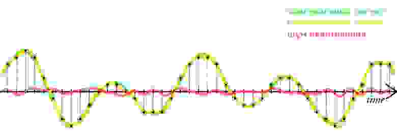
Ошибкой квантований называют отклонение квантованного сигнала от аналогового, т.е. разница между входным значением  и квантованным значением
  (
( )
)
Большие ошибки квантования приводят к сильным искажениям аудиосигнала (шум квантования).
Чем выше разрядность, тем незначительнее ошибки квантования и тем лучше отношение сигнал/шум (Signal-to-noise ratio, SNR), и наоборот: при низкой разрядности вырастает шум (рис. 9).
рис. 9
Разрядность также определяет динамический диапазон сигнала, то есть соотношение максимального и минимального значений. С каждым битом динамический диапазон вырастает примерно на 6dB (Децибел) (6dB это в 2 раза; то есть координатная сетка становиться плотнее, возрастает градация).
рис. 10. Интенсивность шумов при разрядности 6 бит и 8 бит
Ошибки квантования (округления) из-за недостаточного количество уровней не могут быть исправлены.
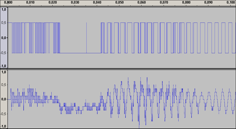
шум квантования
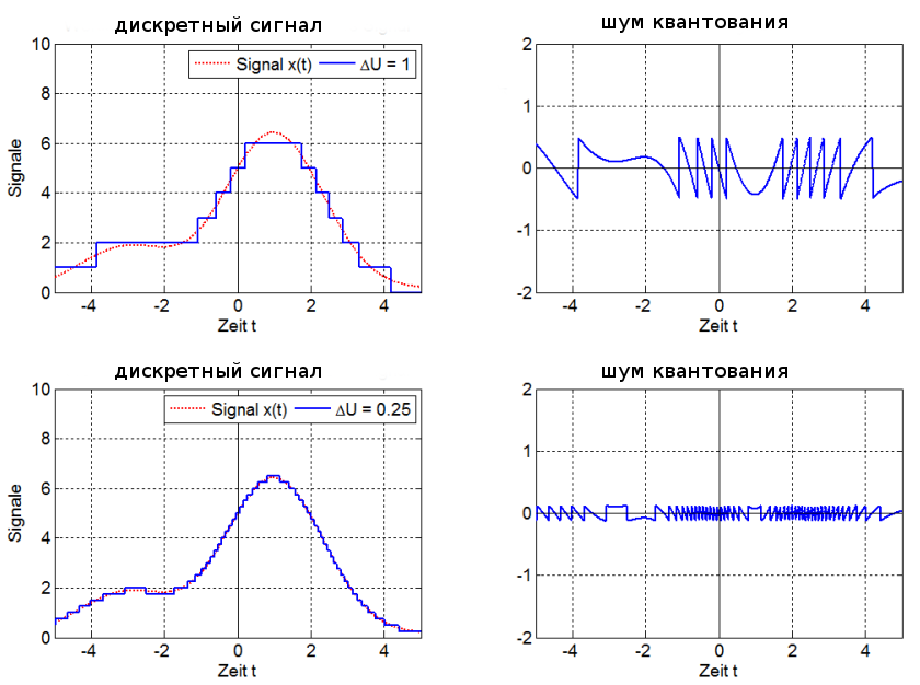
амплитуда сигнала при разрядности 1 бит (сверху) и 4 бит
Аудиопример 1: 8bit/44.1kHz, ~50dB SNR
примечание: если аудиофайлы не воспроизводятся онлайн, пожалуйста, скачивайте их.
Аудиопример 1
Аудиопример 2: 4bit/48kHz, ~25dB SNR
Аудиопример 2
Аудиопример 3: 1bit/48kHz, ~8dB SNR
Аудиопример 3
Теперь о дискретизации.
Как уже говорили ранее, это разбиение сигнала по вертикали и измерение величины значения через определенный промежуток времени. Этот промежуток называется периодом дискретизации или интервалом выборок. Частотой выборок, или частотой дискретизации (всеми известный sample rate) называется величина, обратная периоду дискретизации и измеряется в герцах. Если
T — период дискретизации,
F — частота дискретизации, то

Чтобы аналоговый сигнал можно было преобразовать обратно из цифрового сигнала (точно реконструировать непрерывную и плавную функцию из дискретных, «точечных» значении), нужно следовать теореме Котельникова (теорема Найквиста — Шеннона).
Теорема Котельникова гласит:
Если аналоговый сигнал имеет финитный (ограниченной по ширине) спектр, то он может быть восстановлен однозначно и без потерь по своим дискретным отсчетам, взятым с частотой, строго большей удвоенной верхней частоты.
Вам знакомо число 44.1kHz? Это один из стандартов частоты дискретизации, и это число выбрали именно потому, что человеческое ухо слышит только сигналы до 20kHz. Число 44.1 более чем в два раза больше чем 20, поэтому все частоты в цифровом сигнале, доступные человеческому уху, могут быть преобразованы в аналоговом виде без искажении.
Но ведь 20*2=40, почему 44.1? Все дело в совместимости с стандартами PAL и NTSC. Но сегодня не будем рассматривать этот момент. Что будет, если не следовать теореме Котельникова?
Когда в аудиосигнале встречается частота, которая выше чем 1/2 частоты дискретизации, тогда возникает алиасинг — эффект, приводящий к наложению, неразличимости различных непрерывных сигналов при их дискретизации.
Алиасинг
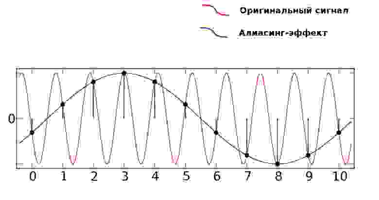
Как видно из предыдущей картинки, точки дискретизации расположены так далеко друг от друга, что при интерполировании (т.е. преобразовании дискретных точек обратно в аналоговый сигнал) по ошибке восстанавливается совершенно другая частота.
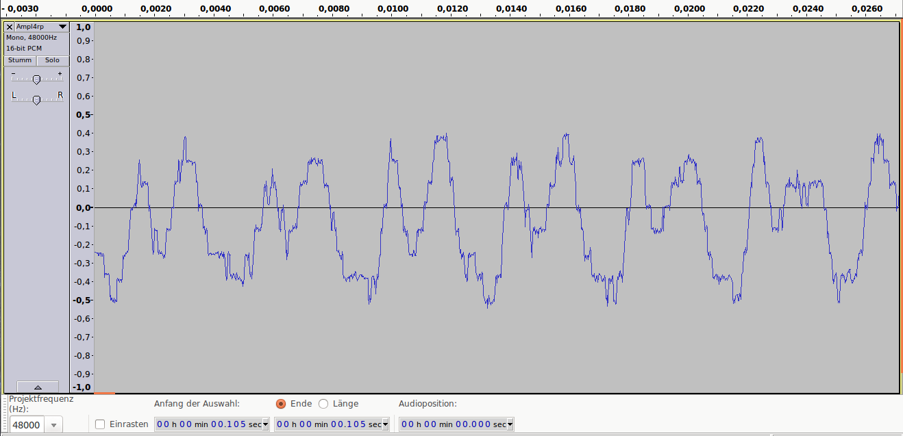
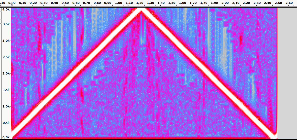
Аудиопример 4: Линейно возрастающая частота от ~100 до 8000Hz. Частота дискретизации — 16000Hz. Нет алиасинга.
Спектральный анализ
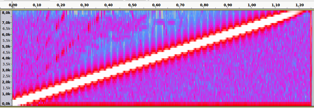
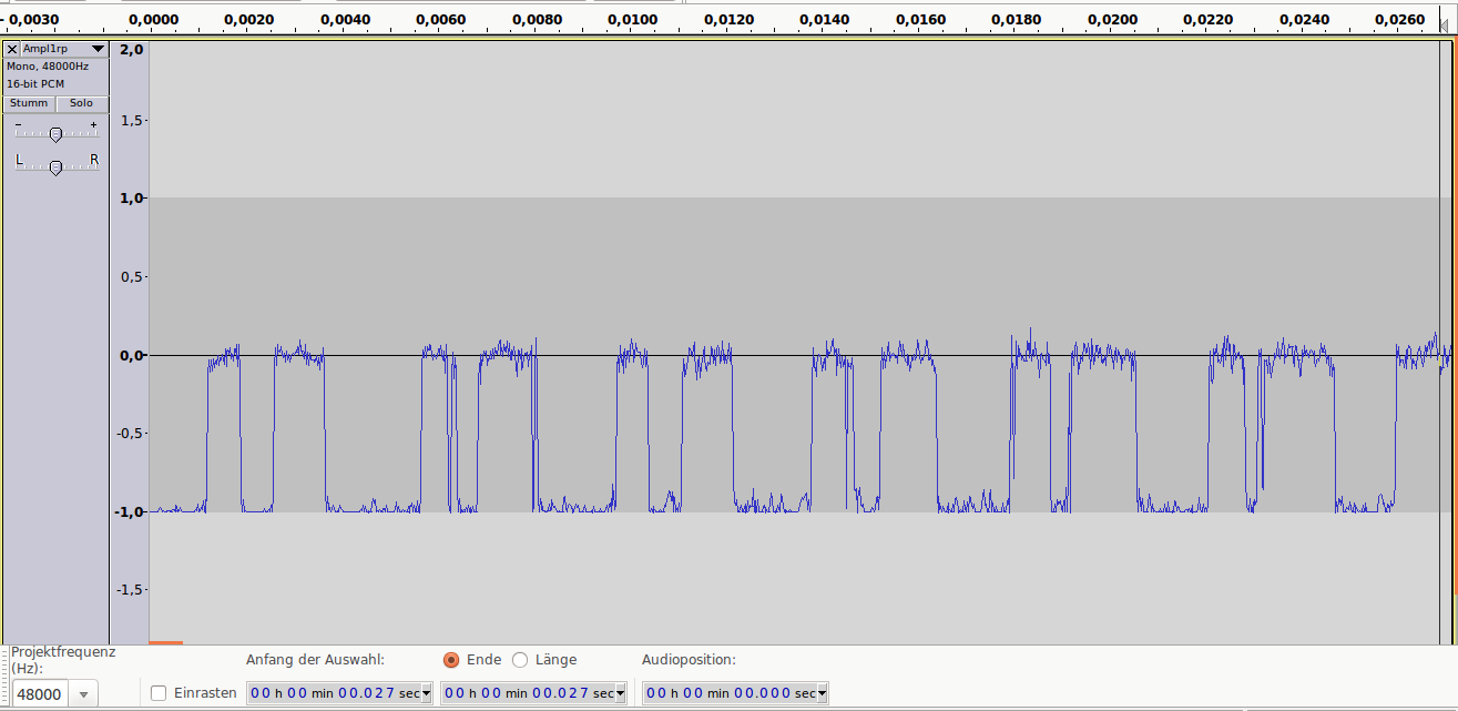
Аудиопример 5: Тот же файл. Частота дискретизации — 8000Hz. Присутствует алиасинг
Спектральный анализ
Пример:
Имеется аудиоматериал, где пиковая частота — 2500Hz. Значит, частоту дискретизации нужно выбрать как минимум 5000Hz.
Следующая характеристика цифрового аудио это битрейт. Битрейт (bitrate) — это объем данных, передаваемых в единицу времени. Битрейт обычно измеряют в битах в секунду (Bit/s или bps). Битрейт может быть переменным, постоянным или усреднённым.
Следующая формула позволяет вычислить битрейт (действительна только для несжатых потоков данных):
Битрейт = Частота дискретизации * Разрядность * Количество каналов
Например, битрейт Audio-CD можно рассчитать так:
44100 (частота дискретизации) * 16 (разрядность) * 2 (количество каналов, stereo)= 1411200 bps = 1411.2 kbit/s
При постоянном битрейте (constant bitrate, CBR) передача объема потока данных в единицу времени не изменяется на протяжении всей передачи. Главное преимущество — возможность довольно точно предсказать размер конечного файла. Из минусов — не оптимальное соотношение размер/качество, так как «плотность» аудиоматериала в течении музыкального произведения динамично изменяется.
При кодировании переменным битрейтом (VBR), кодек выбирает битрейт исходя из задаваемого желаемого качества. Как видно из названия, битрейт варьируется в течение кодируемого аудиофайла. Данный метод даёт наилучшее соотношение качество/размер выходного файла. Из минусов: точный размер конечного файла очень плохо предсказуем.
Усреднённый битрейт (ABR) является частным случаем VBR и занимает промежуточное место между постоянным и переменным битрейтом. Конкретный битрейт задаётся пользователем. Программа все же варьирует его в определенном диапазоне, но не выходит за заданную среднюю величину.
При заданном битрейте качество VBR обычно выше чем ABR. Качество ABR в свою очередь выше чем CBR: VBR > ABR > CBR.
ABR подходит для пользователей, которым нужны преимущества кодирования VBR, но с относительно предсказуемым размером файла. Для ABR обычно требуется кодирование в 2 прохода, так как на первом проходе кодек не знает какие части аудиоматериала должны кодироваться с максимальным битрейтом.
Существуют 3 метода хранения цифрового аудиоматериала:
- Несжатые («сырые») данные
- Данные, сжатые без потерь
- Данные, сжатые с потерями
Несжатый (RAW) формат данных
содержит просто последовательность бинарных значений.
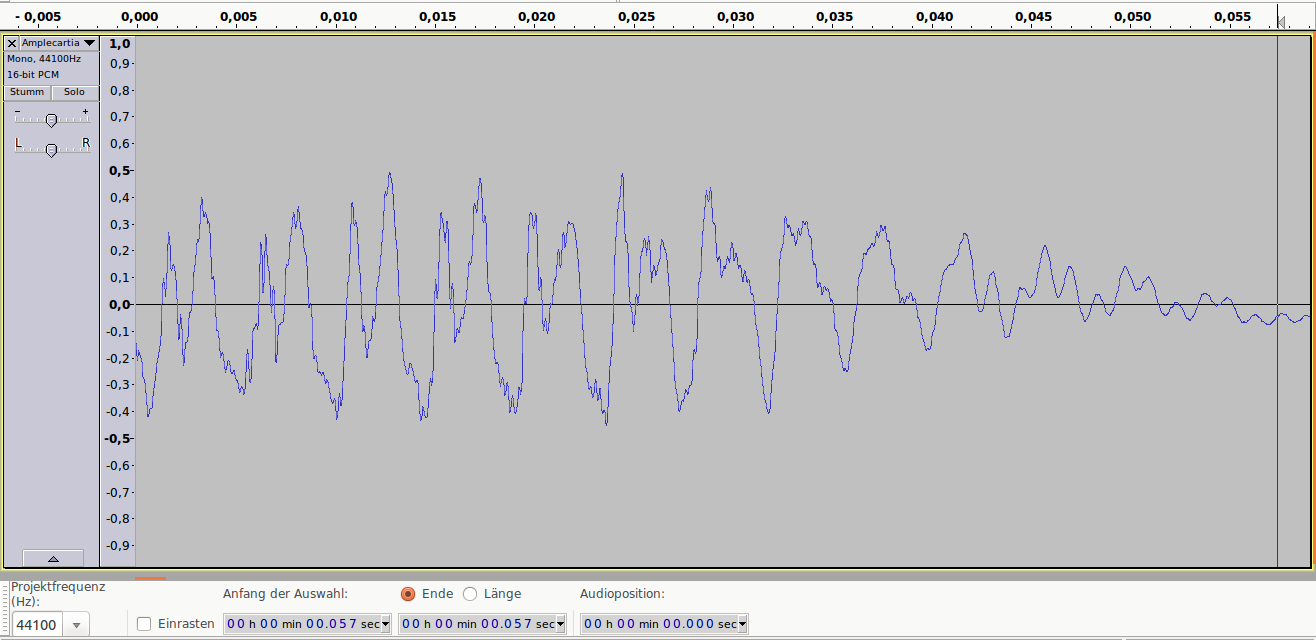
Именно в таком формате хранится аудиоматериал в Аудио-CD. Несжатый аудиофайл можно открыть, например, в программе Audacity. Они имеют расширение .raw, .pcm, .sam, или же вообще не имеют расширения. RAW не содержит заголовка файла (метаданных).
Другой формат хранения несжатого аудиопотока это WAV. В отличие от RAW, WAV содержит заголовок файла.
Аудиоформаты с сжатием без потерь
Принцип сжатия схож с архиваторами (Winrar, Winzip и т.д.). Данные могут быть сжаты и снова распакованы любое количество раз без потери информации.
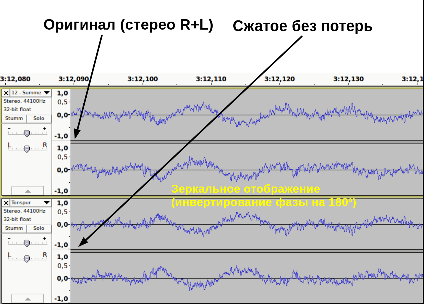
Как доказать, что при сжатии без потерь, информация действительно остаётся не тронутой? Это можно доказать методом деструктивной интерференции. Берем две аудиодорожки. В первой дорожке импортируем оригинальный, несжатый wav файл. Во второй дорожке импортируем тот же аудиофайл, сжатый без потерь. Инвертируем фазу одного из дорожек (зеркальное отображение). При проигрывании одновременно обеих дорожек выходной сигнал будет тишиной.
Это доказывает, что оба файла содержат абсолютно идентичные информации (рис. 11).
рис. 11
Кодеки сжатия без потерь: flac, WavPack, Monkey’s Audio…
При сжатии с потерями
акцент делается не на избежание потерь информации, а на спекуляцию с субъективными восприятиями (Психоакустика). Например, ухо взрослого человек обычно не воспринимает частоты выше 16kHz. Используя этот факт, кодек сжатия с потерями может просто жестко срезать все частоты выше 16kHz, так как «все равно никто не услышит разницу».
Другой пример — эффект маскировки. Слабые амплитуды, которые перекрываются сильными амплитудами, могут быть воспроизведены с меньшим качеством. При громких низких частотах тихие средние частоты не улавливаются ухом. Например, если присутствует звук в 1kHz с уровнем громкости в 80dB, то 2kHz-звук с громкостью 40dB больше не слышим.
Этим и пользуется кодек: 2kHz-звук можно убрать.
Спектральный анализ кодека mp3 с разными уровнями компрессии
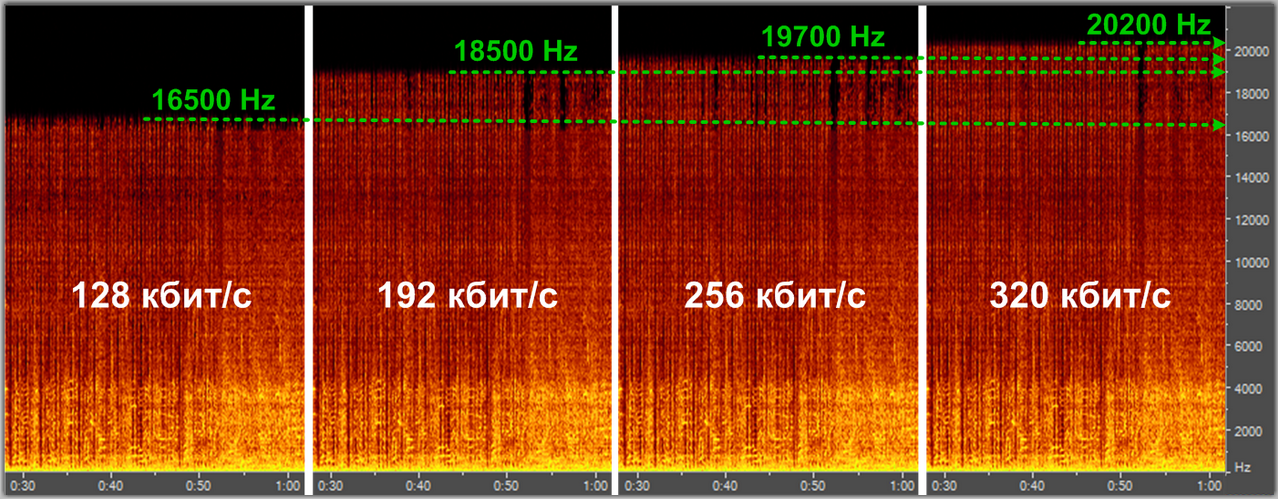
Кодеки сжатия с потерям: mp3, aac, ogg, wma, Musepack…
Спасибо за внимание.
UPD:
Если по каким-либо причинам аудиофайлы не загружаются, можете их скачать здесь: cloud.mail.ru/public/HbzU/YEsT34i4c
Ошибки квантования
В реальных
устройствах цифровой обработки сигналов
необходимо учитывать
эффекты, обусловленные квантованием
входных сигналов
и конечной разрядностью всех регистров.
Источниками ошибок
в процессах обработки сигналов являются
округление (усечение)
результатов арифметических операций,
шум аналого-цифрового квантования
входных аналоговых сигналов, неточность
реализации характеристик цифровых
фильтров из-за округления их коэффициентов
(параметров). В дальнейшем с целью
упрощения анализа предполагается, что
вес источники ошибок независимы и не
коррелируют с входным сигналом (хотя
мы и рассмотрим явление предельных
циклов, обусловленных коррелированным
шумом округления).
Эффект квантования
приводят в конечном итоге к погрешностями выходных сигналах цифровых фильтров
(ЦФ), а в некоторыхслучаяхи к неустойчивым
режимам. Выходную ошибку ЦФ будем
рассчитыватькаксуперпозицию ошибок, обусловленных
каждым независимымисточником.
Квантование
чисел– нелинейная операция;m-разрядное
двоичное числоА
представляетсяb-разрядным
двоичнымчислом
B=F(A),
причем b
< m. В
результате квантования число А
представляется
с ошибкой
е
=B–А= F(А)
–А.
Шаг квантования
Q
=
2–b
определяется весом младшего
числовогоразряда.
При квантовании
используется усечение или округление.
Усечение
числаА
состоит в отбрасываниит
– b
младших разрядов числа, при этом
ошибка усечения
eус=
Fус(А) –А.
Оценим величину
ошибки в предположении m
» b.
Для положительных чисел при любом
способе кодирования –2–b
<еус
0. Для
отрицательных чисел при использовании
прямого и обратного кодов ошибка усечения
неотрицательна: 0еус
< 2–b,
а в дополнительном коде эта ошибка
неположительна: 0еус
> –2–b.
Таким образом, во всех случаях
абсолютное значение ошибки усечения
не превосходит шага квантования:maxeус
< 2–b
=Q.
Округление
m-разрядного
числаA
доb
разрядов (b «
m)b-й
разряд остается неизменным или
увеличивается на единицув
зависимости от соотношения (больше –
меньше) между отбрасываемой дробью
0,аb+1…ат
и величиной
![]() ,
,
гдеаi–i-й
разряд числаA;
i =
b+1,
…,m.
Округление можно практически выполнить
путемприбавления
единицы к (b+1)-му
разряду и усечения полученного числа
до b разрядов.
В таком случае ошибка округления еoк
=
fок(А)–
А
при всех способах кодирования лежит в
пределах
–2–(b+1)
<
еoк
< 2–(b+1)
(1.11)
и, следовательно,
max![]() <2–b
<2–b
= Q/2.
(1.12)
В задачах ЦОС
ошибки квантования чисел рассматриваются
как стационарный
шумоподобный процесс с равномерным
распределением
вероятности по диапазону распределения
ошибок квантования.
(nT)


x(nT)

e(nT)
Рис. 3. Линейная модель квантования
сигналов:
(nT) —дискретный
или m-разрядный
цифровой сигнал (m
> b);
x(nT) —квантованный
b-разрядный
цифровой сигнал;
e(nT)
= x(nT)
–f(nT)
— ошибка
квантования.
Квантование
дискретных сигналов состоит в
представлении отсчета
(выборки сигнала) числамиx(nT),
содержащими b
числовых разрядов. Квантование сигналов,
как и квантование
чисел – нелинейная операция. Однако
при анализе процессов в ЦФ целесообразно
использовать линейную модель квантования
сигналов – рис. 3.
Верхнее значение ошибки квантования
![]() определяетсясоотношением
определяетсясоотношением
(1.11) или (1.12).
Вероятностные
оценки ошибок квантования основаны на
предположениях о том, что
последовательностье(пТ)являетсястационарным
случайным процессом с равномерным
распределением вероятности по
диапазону ошибок квантования ие(пТ)
не коррелирован
с f(nT).
Математическое
ожидание (среднее значение) e
и дисперсия
![]() ошибки квантованияе
ошибки квантованияе
определяются
по формулам:
![]() =E(е)
=E(е)
=![]() ,
,
![]() =
=![]() =
=![]() =E(е2)
=E(е2)
–![]() ,
,
где ре
— плотность вероятности ошибки. По
этим формуламвычисляются
математическое ожидание и дисперсия
для ошибок
округления и усечения:
![]() =
=
![]() =
=
![]()
В логарифмическоммасштабе
![]() =
=![]()
Лекция 2