Функция если ошибка в vba excel

VBA IFERROR

A written code many times gives the error and chances of getting an error in complex error are quite high. Like excel has IFERROR function which is used where there are chances of getting an error. IFERROR changes the error message into other text statements as required and defined by the user. Similarly, VBA IFERROR functions same as the IFERROR function of Excel. It changes the error message into the defined text by the user.

This error mostly occurs when we perform any mathematical function or if we are mapping any data which is in a different format. IFERROR handles many errors, some of them are:

#VALUE!, #N/A, #DIV/0!, #REF!, #NUM!, #NULL! And #NAME?

Example #1

Now this IFERROR function can also be implemented in VBA. Now to compare the results from Excel with VBA IFERROR we will insert a column where we will apply VBA IFERROR statement as shown below.

You can download this VBA IFERROR Excel Template here – VBA IFERROR Excel Template

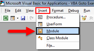
For this, we consider the same data and insert another column where we will perform VBA IFERROR. Go to VBA window and insert a new Module from Insert menu as shown below.

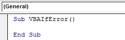
Now in a newly opened module, write Sub-category with any name. Here we have given the name of the operating function as shown below.

Code:

Sub VBA_IfError()
End Sub

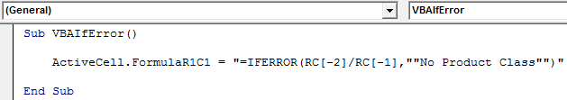
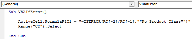
Now with the help of ActiveCell, we will select the first reference cell and then directly use IFERROR Formula with reference cell (RC) -2 divided by -1 cell numbers. Which means we are dividing cell A by cell B in the first argument. And in the second argument write any statement which we want in place of error. Here we will use the same state which we have seen above i.e. “No Product Class”.

Code:

Sub VBA_IfError()

    ActiveCell.FormulaR1C1 = "=IFERROR(RC[-2]/RC[-1],""No Product Class"")"

End Sub

Now select the range cell which would be our denominator. Here we have selected cell C2.

Code:

Sub VBA_IfError()

    ActiveCell.FormulaR1C1 = "=IFERROR(RC[-2]/RC[-1],""No Product Class"")"
    Range("C2").Select

End Sub

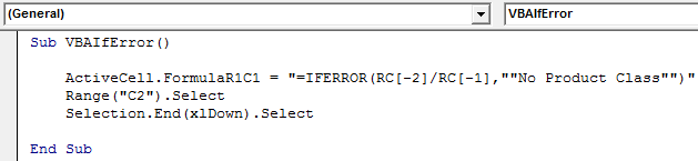
Now to drag the formula to below cells where we need to apply IFERROR till the table has the values.

Code:

Sub VBA_IfError()

    ActiveCell.FormulaR1C1 = "=IFERROR(RC[-2]/RC[-1],""No Product Class"")"
    Range("C2").Select
    Selection.End(xlDown).Select

End Sub

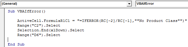
Now to come to the last cell of the column with the help of command Range where we need to drag the IFERROR formula. Here our limit ends at cell D6.

Code:

Sub VBA_IfError()

    ActiveCell.FormulaR1C1 = "=IFERROR(RC[-2]/RC[-1],""No Product Class"")"
    Range("C2").Select
    Selection.End(xlDown).Select
    Range("D6").Select

End Sub

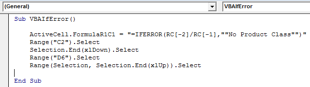
Now to drag the applied IFERROR down to all the applicable cells select the Range from End (or Last) cell to Up to the applied formula cell by End(xlUp) command under Range.

Code:

Sub VBA_IfError()

    ActiveCell.FormulaR1C1 = "=IFERROR(RC[-2]/RC[-1],""No Product Class"")"
    Range("C2").Select
    Selection.End(xlDown).Select
    Range("D6").Select
    Range(Selection, Selection.End(xlUp)).Select

End Sub

As we do Ctrl + D to drag the up cell values to all selected cells in excel, here in VBA, Selection.FillDown is used to fill the same up cells values in all selected cells.

Code:

Sub VBA_IfError()

    ActiveCell.FormulaR1C1 = "=IFERROR(RC[-2]/RC[-1],""No Product Class"")"
    Range("C2").Select
    Selection.End(xlDown).Select
    Range("D6").Select
    Range(Selection, Selection.End(xlUp)).Select
    Selection.FillDown

End Sub

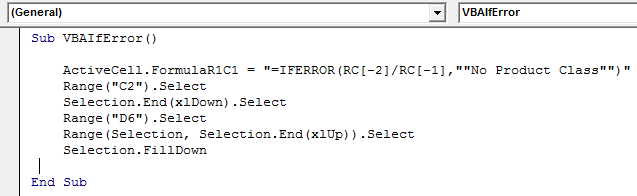
This completes the coding of VBA IFERROR. Now run the complete code by clicking on the play button as shown in below screenshot.

As we can see above, in column D starting from Cell 2 to 6 we got our results.

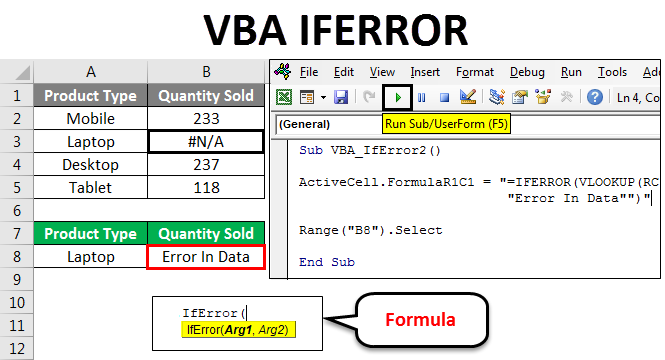
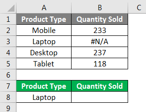
There is another format and way to apply IFERROR in VBA. For this, we will consider another set of data as shown below. Below we have sales data of some products in column A and quality sold in column B. And we need map this data at cell F2 with reference to product type Laptop. Now data in the first table has #N/A in cell B3 with for Laptop quantity sold out which means that source data itself has an error. And if we look up the data from the first table to Cell F2 we will get same #N/A here.

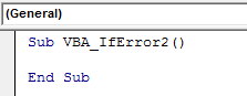
For this open a new module in VBA and write Subcategory with the name of a performed function.

Code:

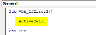
Sub VBA_IfError2()

End Sub

Select range where we need to see the output or directly activate that cell by ActiveCell followed by dot (.) command line as shown below.

Code:

Now select FormulaR1C1 from the list which is used for inserting any excel function.

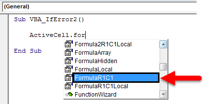
Now use the same formula as used in excel function in VBA as well.

Code:

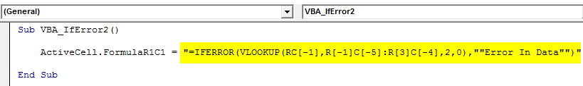
Sub VBA_IfError2()

    ActiveCell.FormulaR1C1 = "=IFERROR(VLOOKUP(RC[-1],R[-1]C[-5]:R[3]C[-4],2,0),""Error In Data"")"

End Sub

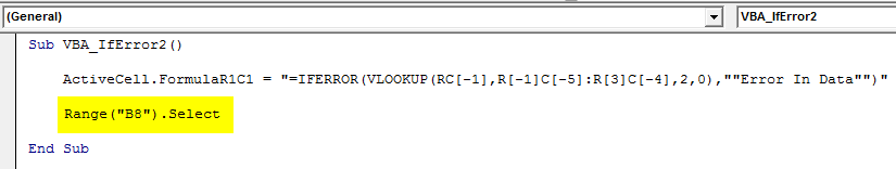
Now select the cell where we need to see the output in Range. Here we have selected cell F3.

Code:

Sub VBA_IfError2()

    ActiveCell.FormulaR1C1 = "=IFERROR(VLOOKUP(RC[-1],R[-1]C[-5]:R[3]C[-4],2,0),""Error In Data"")"

    Range("B8").Select

End Sub

Now compile and run complete code using F5 key or manually and see the result as shown below.

As we can see in the above screenshot, the output of product type Laptop, from first table #N/A is with error text “Error In Data” as defined in VBA code.

Pros of VBA IFERROR Function

It takes little time to apply the IFERROR function through VBA.
Result from Excel insert function and VBA IFERROR coding, both are the same.
We can format or paste special the applied formula as well to avoid any further problem.

Cons of VBA IFERROR Function

IFERROR with this method, referencing the range of selected cell may get disturbed as the table has limited cells.

Things To Remember

We can record the macro and modify the recorded coding as per our need.
Always remember to save the file as Macro-Enabled Excel, so that we can use the applied or created macro multiple times without any issue.
Make sure you remember to compile the complete code before ending the command function. By this, we can avoid or correct any error incurred.
You can apply the created code into a button or tab and use it by a single click. This is the quickest way to run the code.
Best way to avoid any changes after running the code is to paste special the complete cells so that there will not be any formula into the cell.

Errors Happen

We may come across several functions in programming languages. In VBA, we are prone to encounter errors like:

Syntax errors
Compile time errors
Runtime errors

These are errors in code which can be handled using error handling methods. For example, you can see some best practices in articles like this one.

In this article, we will discuss some logical errors which will give unexpected output.

Example Scenario

Let us try to copy the contents of a cell to another while the data in the cell has invalid or improper data like a “DIV/0” error which we are not aware of.

In this case, the contents would simply get pasted as-is. But we do not want to use this erroneous data in another sheet or any cell in the same sheet.

In that case, we need an option wherein the copy paste happens only if the source data is error-free. In case of error, we need some specific statement to be pasted there.

The IfError function of VBA can help us achieve this easily.

IfError Function

The IfError function can help point out/display obvious errors in other functions that may not catch our eye easily.

This function is used to prevent mathematical errors or any other errors that occur from a copy paste action when the source value or the resulting value has an error. This function displays resulting values only if they are error-free. If there are errors in the output values, an alternate statement text is displayed.

Syntax:

IfError( < source value> , <alternate text> )

Where:

<source value> is the cell from which text is copied
<alternate text> is the statement to be used in case the value of source text is erroneous.

Paste One Column’s Cell Values to Another With and Without the IfError Function

Sub ifferror_demo()
'just a for loop to iterate through each row starting from 1 to 20
For i = 1 To 20
' simply paste the cell values of col 4 to col 6
Cells(i, 6).Value = Cells(i, 4).Value
&<pre&>&<code&>' paste the values of col 4 to col 6 only if the values have no errors. If not "invalid numbers" will be pasted.
Cells(i, 5).Value = WorksheetFunction.IfError(Cells(i, 4).Value, "Invalid numbers")&>/code&>&</pre&>;
Next
End Sub

The image above shows the difference between the simple paste and paste data using the “IfError” function in VBA.

The data in column E pasted using the IfError function looks reasonable and clear.

But the data in col F that has been pasted without using the “IfError” function has not corrected/checked anything for us.

Program That Uses IfError With Vlookup

In this program, we will try to see the price/piece of any item that is selected from a list in a cell.

Price/piece is in col D and the item is in col A. So, we will use “vlookup” here.

I’m setting data validation to list the items in cell H4.

For this, we can go to Data tab-> Data tools-> Data validation.

Choose a list and select the range as the source.

The items are now listed here:

Now I apply the vlookup formula to get the price/piece of the selected item.

Now I select some item from the list in cell H4 that has a “Division by 0 error” in col D, eg: Cake.

To avoid this kind of output, we have to use the “IfError” formula, which can filter out these errors and display a value that the viewers can understand.

Here, the existing vlookup formula is wrapped in an “IfError” formula with the vlookup formula as the first argument. The second argument is an alternate text to be displayed in case the result is erroneous.

The proper value would be displayed in case the output is error-free.

Do the same using a macro code (VBA):

Sub Excel_IFERROR_demo()

' declare a variable of type worksheet
Dim ws As Worksheet
' assign the worksheet
Set ws = Worksheets("Snackbar")

' apply the Excel IFERROR function with the vlookup function
ws.Range("I4") = Application.WorksheetFunction.IfError(Application.VLookup(ws.Range("H4").Value, ws.Range("A1:D13"), 4, False), "CHECK THE VALUE")

End Sub

Now, we will delete the formula in cell “I4” and use this macro to fill the data in that cell.

What does this code do?

This declares a worksheet object, assigns the worksheet to it. Then, we assign the vlookup formula to the cell I4 . The formula depends on the value in cell H4.

Whenever we change the value in cell H4, this code should be run to fill the corresponding value in cell I4.

A couple of output results to demonstrate how this code works:

A Program for Mathematical Calculation

This program is for direct division or calculation of price/piece for the item “Roti.”

Sub Excel_IFERROR_demo_2()

' declare a variable of type worksheet
Dim ws As Worksheet
' assign the worksheet
Set ws = Worksheets("Snackbar")

' apply the Excel IFERROR function with the vlookup function
ws.Range("D7") = Application.WorksheetFunction.IfError(ws.Range("B7").Value / ws.Range("C7").Value, "CHECK THE VALUE")

End Sub

Here the formula =B7/C6 in the cell D7 is replaced by the output of this code.

A couple of output values for corresponding input values.

Note: Change the values of B7 or C7 or both and run this procedure (code) to see the output in D7.

Summary

“IfError” is available both as a formula and VBA function in Microsoft Excel. This helps us catch the logical faults (e.g.: Math calculations) and not the syntax or compile errors. They are mostly used in Excel formulae directly instead of macros. In the case of automated macro utilities that are large in size, they can be used in the respective VBA code too.

Tagged with: Error, error handling, Errors, Excel, Functions, IfError, Macro, macro code, VBA, VBA For Excel, worksheet functions

Источник

Точно так же, как мы используем ЕСЛИОШИБКА в excel, чтобы знать, что делать, когда ошибка встречается перед каждой функцией, у нас есть встроенная функция ЕСЛИОШИБКА в VBA, которая используется таким же образом, поскольку это функция рабочего листа, мы используем эту функцию с рабочим листом. в VBA, а затем мы предоставляем аргументы для функции.

Функция ЕСЛИОШИБКА в VBA

Ожидать, что код будет работать без каких-либо ошибок, — преступление. Для обработки ошибок в VBA у нас есть несколько способов использования таких операторов, как On Error Resume Next VBA, On Error Resume Goto 0, On Error GoTo Label. Обработчики ошибок VBA могут перейти только к следующей строке кода. Но в случае, если вычисление не происходит, нам нужно заменить ошибку другим идентифицирующим словом. В этой статье мы увидим, как этого добиться с помощью функции VBA IFERROR в excel.

Как использовать ЕСЛИОШИБКА в VBA?

Здесь следует помнить, что это не функция VBA, а просто функция рабочего листа.

Вы можете скачать этот шаблон Excel для VBA IFERROR здесь — Шаблон Excel для VBA IFERROR

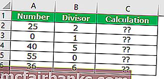
Например, приведенные выше данные возьмите только для демонстрации.

Шаг 1. Определите переменную как целое число .

Код:

 Sub Iferror_Example1 () Dim i As Integer End Sub

Шаг 2: Чтобы выполнить расчет, откройте For Next Loop .

Код:

 Sub Iferror_Example1 () Dim i As Integer For i = 2–6 Next i End Sub

Шаг 3: внутри напишите код как Cells (I, 3) .Value =

Код:

 Sub Iferror_Example1 () Dim i как целое число для i = от 2 до 6 ячеек (i, 3). Value = Next i End Sub

Шаг 4: Чтобы получить доступ к функции ЕСЛИОШИБКА, мы не можем просто ввести формулу, нам нужно использовать класс «WorksheetFunction» .

Код:

 Sub Iferror_Example1 () Dim i как целое число для i = от 2 до 6 ячеек (i, 3) .Value = WorksheetFunction.If Next i End Sub

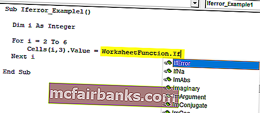
Шаг 5: Как вы можете видеть на изображении выше, после вставки класса команды «WorksheetFunction» мы получаем формулу ЕСЛИОШИБКА. Выберите формулу.

Код:

 Sub Iferror_Example1 () Dim i как целое число для i = от 2 до 6 ячеек (i, 3) .Value = WorksheetFunction.IfError (Next i End Sub

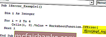
Шаг 6: Одна из проблем в VBA при доступе к функциям рабочего листа, мы не видим аргументов, подобных тем, которые мы видели на рабочем листе. Вы должны быть абсолютно уверены в аргументах, которые мы используем.

По этой причине, прежде чем я покажу вам ЕСЛИОШИБКУ в VBA, я показал вам синтаксис функции рабочего листа.

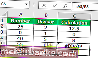
Первым аргументом здесь является «Значение», т.е. какую ячейку вы хотите проверить. Перед этим примените расчет в ячейке.

Теперь в VBA примените приведенные ниже коды.

Код:

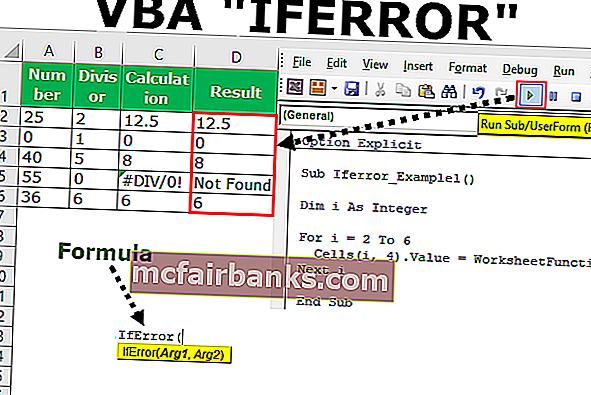
 Sub Iferror_Example1 () Dim i как целое число для i = от 2 до 6 ячеек (i, 4) .Value = WorksheetFunction.IfError (Cells (i, 3) .Value, «Not Found») Next i End Sub

Теперь функция ЕСЛИОШИБКА проверяет наличие ошибок в столбце C, и при обнаружении ошибок в столбце D отображается результат «Не найдено».

Подобно этому, используя функцию ЕСЛИОШИБКА, мы можем изменить результаты по нашему желанию. В этом случае я изменил результат на «Не найдено». Вы можете изменить это по своему усмотрению.

Типы ошибок, которые можно найти в VBA IFERROR

Важно знать типы ошибок Excel, которые может обрабатывать функция ЕСЛИОШИБКА. Ниже приведены типы ошибок, которые может обрабатывать ЕСЛИОШИБКА.

# N / A, #VALUE !, #REF !, # DIV / 0 !, #NUM !, #NAME? Или #NULL !.

Источник

Содержание

Обзор функции ЕСЛИОШИБКА
Что такое функция ЕСЛИОШИБКА?
Дополнительные примеры формул ЕСЛИОШИБКА
ЕСЛИ ОШИБКА в Google Таблицах
ЕСЛИОШИБКА Примеры в VBA

В этом руководстве показано, как использовать функцию Excel ЕСЛИОШИБКА для обнаружения ошибок формулы, заменяя их другой формулой, пустым значением, 0 или настраиваемым сообщением.

Обзор функции ЕСЛИОШИБКА

Функция ЕСЛИОШИБКА Проверяет, приводит ли формула к ошибке. Если ЛОЖЬ, вернуть исходный результат формулы. Если ИСТИНА, вернуть другое указанное значение.

ЕСЛИОШИБКА Синтаксис

Чтобы использовать функцию таблицы Excel ЕСЛИОШИБКА, выберите ячейку и введите:
= ЕСЛИОШИБКА (
Обратите внимание, как появляются входные данные формулы ЕСЛИОШИБКА:

Синтаксис и входные данные функции ЕСЛИОШИБКА:

1	= ЕСЛИОШИБКА (ЗНАЧЕНИЕ; значение_если_ошибка)

ценить — Выражение. Пример: 4 / A1

value_if_error — Значение или расчет для выполнения, если предыдущий ввод привел к ошибке. Пример 0 или «» (пусто)

Что такое функция ЕСЛИОШИБКА?

Функция ЕСЛИОШИБКА относится к категории логических функций в Microsoft Excel, которая включает ISNA, ISERROR и ISERR. Все эти функции помогают обнаруживать и обрабатывать ошибки формул.

ЕСЛИОШИБКА позволяет выполнить расчет. Если расчет не приведет к ошибке, затем отобразится результат расчета. Если расчет делает приводит к ошибке, тогда выполняется другое вычисление (или выводится статическое значение, такое как 0, пробел или какой-то текст).

Когда бы вы использовали функцию ЕСЛИОШИБКА?

При делении чисел во избежание ошибок, связанных с делением на 0
При выполнении поиска для предотвращения ошибок, если значение не найдено.
Если вы хотите выполнить другое вычисление, если первое приводит к ошибке (например, поиск значения в 2^nd table, если его нет в первой таблице)

Необработанные ошибки формул могут вызвать ошибки в вашей книге, но видимые ошибки также делают вашу электронную таблицу менее привлекательной.

Если ошибка, то 0

Давайте посмотрим на простой пример. Ниже вы делите два числа. Если вы попытаетесь разделить на ноль, вы получите сообщение об ошибке:

Вместо этого вставьте вычисление в функцию ЕСЛИОШИБКА, и если вы разделите на ноль, вместо ошибки будет выведено 0:

1	= ЕСЛИОШИБКА (A2 / B2; 0)

Если ошибка, то пусто

Вместо того, чтобы устанавливать для ошибок значение 0, вы можете установить их как «пустые» с двойными кавычками («»):

1	= ЕСЛИОШИБКА (A2 / B2; «»)

Мы рассмотрим больше случаев использования ЕСЛИОШИБКИ с функцией ВПР …

ЕСЛИ ОШИБКА с ВПР

Функции поиска, такие как VLOOKUP, будут генерировать ошибки, если значение поиска не будет найдено. Как показано выше, вы можете использовать функцию ЕСЛИОШИБКА для замены ошибок пробелами («») или нулями:

1	= ЕСЛИОШИБКА (ВПР (A2, LookupTable1! $ A $ 2: $ B $ 4,2; FALSE), «не найдено»)

Если ошибка, то сделайте что-нибудь еще

Функцию ЕСЛИОШИБКА также можно использовать для выполнения второго вычисления, если первое вычисление приводит к ошибке:

12	= ЕСЛИОШИБКА (ВПР (A2; LookupTable1! $ A $ 2: $ B $ 4,2; FALSE),ВПР (A2, LookupTable2! $ A $ 2: $ B $ 4,2, FALSE))

Здесь, если данные не найдены в «LookupTable1», вместо этого выполняется ВПР для «LookupTable2».

Дополнительные примеры формул ЕСЛИОШИБКА

Вложенная ЕСЛИОШИБКА — ВПР на нескольких листах

Вы можете вложить ЕСЛИОШИБКУ в другую ЕСЛИОШИБКА, чтобы выполнить 3 отдельных вычисления. Здесь мы будем использовать два IFERROR для выполнения ВПР на 3 отдельных листах:

123	= ЕСЛИОШИБКА (ВПР (A2; LookupTable1! $ A $ 2: $ B $ 4,2; FALSE),ЕСЛИОШИБКА (ВПР (A2; LookupTable2! $ A $ 2: $ B $ 4,2; FALSE),ВПР (A2, LookupTable3! $ A $ 2: $ B $ 4,2, FALSE)))

Индекс / соответствие и XLOOKUP

Конечно, IFERROR также будет работать с формулами Index / Match и XLOOKUP.

ЕСЛИ ОШИБКА XLOOKUP

Функция XLOOKUP — это расширенная версия функции VLOOKUP.

1	= ЕСЛИОШИБКА (XLOOKUP (A2, LookupTable1! $ A $ 2: $ A $ 4, LookupTable1! $ B $ 2: $ B $ 4), «Не найдено»)

ИНДЕКС ЕСЛИ ОШИБКА / СООТВЕТСТВИЕ

ИНДЕКС и ПОИСКПОЗ можно использовать для создания более мощных ВПР (аналогично тому, как работает новая функция XLOOKUP) в Excel.

1	= ЕСЛИОШИБКА (ИНДЕКС (LookupTable1! $ B $ 2: $ B $ 4, MATCH (A3, LookupTable1! $ A $ 2: $ A $ 4,0)), «Не найдено»)

ЕСЛИОШИБКА в массивах

Формулы массива в Excel используются для выполнения нескольких вычислений с помощью одной формулы. Предположим, есть три столбца: Год, Продажи и Средняя цена. Вы можете узнать общее количество по следующей формуле в столбце E.

1	{= СУММ ($ B $ 2: $ B $ 4 / $ C $ 2: $ C $ 4)}

Формула работает хорошо до тех пор, пока она не попытается разделить на ноль, в результате чего получится # DIV / 0! ошибка.

Вы можете использовать функцию ЕСЛИОШИБКА для устранения ошибки следующим образом:

1	{= СУММ (ЕСЛИОШИБКА ($ B $ 2: $ B $ 4 / $ C $ 2: $ C $ 4,0))}

Обратите внимание, что функция ЕСЛИОШИБКА должна быть вложена в функцию СУММ, иначе ЕСЛИОШИБКА будет применяться к общей сумме, а не к каждому отдельному элементу в массиве.

IFNA против ЕСЛИ ОШИБКА

Функция IFNA работает точно так же, как функция ЕСЛИОШИБКА, за исключением того, что функция IFNA выявляет только ошибки # Н / Д. Это чрезвычайно полезно при работе с функциями поиска: обычные ошибки формул по-прежнему будут обнаруживаться, но ошибки не появятся, если значение поиска не найдено.

1	= IFNA (ВПР (A2; LookupTable1! $ A $ 2: $ B $ 4,2; FALSE); «Не найдено»)

Если ISERROR

Если вы все еще используете Microsoft Excel 2003 или более старую версию, вы можете заменить IFERROR комбинацией IF и ISERROR. Вот краткий пример:

1	= ЕСЛИ (ЕСТЬ ОШИБКА (A2 / B2); 0; A2 / B2)

Функция ЕСЛИОШИБКА работает в Google Таблицах точно так же, как и в Excel:

ЕСЛИОШИБКА Примеры в VBA

VBA не имеет встроенной функции ЕСЛИОШИБКА, но вы также можете получить доступ к функции ЕСЛИОШИБКА Excel из VBA:

12	Dim n до тех пор, покаn = Application.WorksheetFunction.IfError (Значение, значение_если_ошибка)

Application.WorksheetFunction дает вам доступ ко многим (не всем) функциям Excel в VBA.

Обычно ЕСЛИОШИБКА используется при чтении значений из ячеек. Если ячейка содержит ошибку, VBA может выдать сообщение об ошибке при попытке обработать значение ячейки. Попробуйте это с помощью приведенного ниже примера кода (где ячейка B2 содержит ошибку):

1234567891011

Sub IFERROR_VBA ()Dim n по длине, м по длинеЕСЛИ ОШИБКАn = Application.WorksheetFunction.IfError (Диапазон («b2»). Значение, 0)«Нет ЕСЛИОШИБКИm = Диапазон («b2»). ЗначениеКонец подписки

Код присваивает ячейку B2 переменной. Второе присвоение переменной вызывает ошибку, потому что значение ячейки # Н / Д, но первое работает нормально из-за функции ЕСЛИОШИБКА.

Вы также можете использовать VBA для создания формулы, содержащей функцию ЕСЛИОШИБКА:

1	Диапазон («C2»). FormulaR1C1 = «= ЕСЛИОШИБКА (RC [-2] / RC [-1], 0)»

Обработка ошибок в VBA сильно отличается от обработки ошибок в Excel. Обычно для обработки ошибок в VBA используется обработка ошибок VBA. Обработка ошибок VBA выглядит так:

12345678910111213141516171819

Sub TestWS ()MsgBox DoesWSExist («тест»)Конец подпискиФункция DoesWSExist (wsName As String) As BooleanDim ws как рабочий листПри ошибке Возобновить ДалееУстановить ws = Sheets (wsName)’Если ошибка WS не существуетЕсли Err.Number 0, тоDoesWSExist = FalseЕщеDoesWSExist = TrueКонец, еслиПри ошибке GoTo -1Конечная функция

Обратите внимание, что мы используем Если Err.Number 0, то чтобы определить, произошла ли ошибка. Это типичный способ отлова ошибок в VBA. Однако функция ЕСЛИОШИБКА имеет некоторые применения при взаимодействии с ячейками Excel.

Источник

VBA IFERROR

Pros of VBA IFERROR Function

Cons of VBA IFERROR Function

Things To Remember

Recommended Articles

Errors Happen

Example Scenario

IfError Function

Paste One Column’s Cell Values to Another With and Without the IfError Function

Program That Uses IfError With Vlookup

A Program for Mathematical Calculation

Summary

Функция ЕСЛИОШИБКА в VBA

Как использовать ЕСЛИОШИБКА в VBA?

Типы ошибок, которые можно найти в VBA IFERROR

Обзор функции ЕСЛИОШИБКА

ЕСЛИОШИБКА Синтаксис

Синтаксис и входные данные функции ЕСЛИОШИБКА:

Что такое функция ЕСЛИОШИБКА?

Если ошибка, то 0

Если ошибка, то пусто

ЕСЛИ ОШИБКА с ВПР

Если ошибка, то сделайте что-нибудь еще

Дополнительные примеры формул ЕСЛИОШИБКА

Вложенная ЕСЛИОШИБКА — ВПР на нескольких листах

Индекс / соответствие и XLOOKUP

ЕСЛИ ОШИБКА XLOOKUP

ИНДЕКС ЕСЛИ ОШИБКА / СООТВЕТСТВИЕ

ЕСЛИОШИБКА в массивах

IFNA против ЕСЛИ ОШИБКА

Если ISERROR

ЕСЛИОШИБКА Примеры в VBA

Возможно, вам также будет интересно: