Ignore the Excel error or update your formula to include the cells
by Claire Moraa
Claire likes to think she’s got a knack for solving problems and improving the quality of life for those around her. Driven by the forces of rationality, curiosity,… read more
Updated on December 14, 2022
Reviewed by
Alex Serban

After moving away from the corporate work-style, Alex has found rewards in a lifestyle of constant analysis, team coordination and pestering his colleagues. Holding an MCSA Windows Server… read more
- The error formula omits adjacent cells means that Excel cannot calculate the formula because it is missing something.
- Excel tries to calculate a formula but only takes into account the values from one cell, ignoring other cells with values needed for the calculation.
- If this happens, it means that you have left out a cell on one side of your formula and need to clean up your sheet.
XINSTALL BY CLICKING THE DOWNLOAD FILE
This software will repair common computer errors, protect you from file loss, malware, hardware failure and optimize your PC for maximum performance. Fix PC issues and remove viruses now in 3 easy steps:
- Download Restoro PC Repair Tool that comes with Patented Technologies (patent available here).
- Click Start Scan to find Windows issues that could be causing PC problems.
- Click Repair All to fix issues affecting your computer’s security and performance
- Restoro has been downloaded by 0 readers this month.
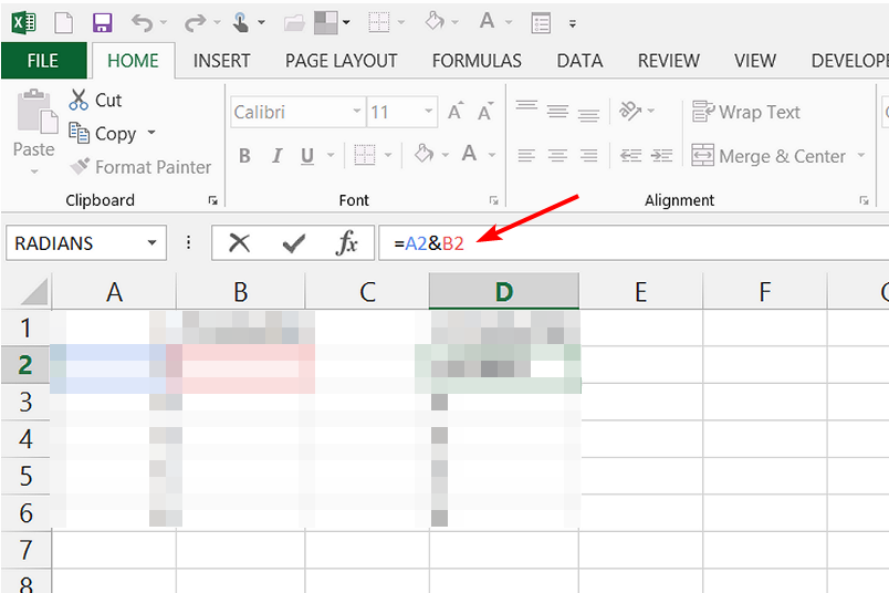
If you get an error message saying that your formula omits adjacent cells when you try to enter it, your Excel spreadsheet has probably been modified.
The problem is that when such an error occurs, it can mess up your entire worksheet. You may have to redo all of your calculations from scratch or worse, start over, especially if Excel fails to respond when saving.
What does the error formula omits adjacent cells mean in excel?
The error formula omits adjacent cells means that there is an error in the formula in the cell. When you have an array of formulas, Excel assumes that the data for all are continuous and not separated by other data.
If your data is separated by other data or if some cells contain blank values, then Excel will not be able to evaluate the formula correctly. But why does this happen? Below are some possible reasons:
- Cell has no data – The error function in Excel only calculates values for cells where there is data present. If a cell has no data, then it will not be included in the calculation process.
- The cell no longer exists – It is possible that the formula you may be referencing belongs to a cell that has been deleted or renamed.
- Range has been changed – The formula may be referencing a dynamic range that no longer exists due to changes in the spreadsheet.
- Blank cells in between – This error occurs when there are empty cells between each cell that you want to include in your formula.
What can I do if the Excel error formula omits adjacent cells?
Check off the following first before you proceed:
- First, check to make sure that your formula includes all of the necessary parts.
- If you are working with a small data set, try to identify any empty cells and delete them.
1. Uncheck formulas that omit cells
- Launch your Excel sheet and then click on File.
- Navigate to Options and then select Formulas.

- Look for Error checking rules and uncheck Formulas which omit cells in a region.

- Click OK.
2. Switch from absolute to relative reference
- Open the Excel sheet and select the cell that contains the formula.
- Navigate to the formula bar at the top and press F4 until you get the relative reference option.

Absolute and relative references in Excel formulas are two ways to refer to cells in your spreadsheet. They both have their purpose, and sometimes you may find yourself using them interchangeably.
Absolute cell references are the default in Excel. However, there are times when using an absolute reference is not the best option. This type of notation is not always intuitive because it does not take into account the position of the cell that contains the formula.
- Runtime Error 57121: Application-Defined or Object-Defined [Fix]
- Runtime Error 7: Out of Memory [Fix]
- MegaStat for Excel: How to Download & Install
3. Update the formula to include the cells
When you update the formula to include the cells that you want to reference, Excel can properly evaluate it and display its result properly.
The caveat to this method is that if you have a very large spreadsheet with many formulas, then it can be difficult to track down which cell is causing the problem.
If nothing seems to work, you can opt to ignore the error or seek help from the help task pane in Excel. The built-in tool diagnoses some problems and may be able to recommend a solution.
Excel errors are in no shortage as you can expect to encounter a few hiccups when you’re working with sheets and formulas. We have crafted a dedicated article to help you in case you want to recover a corrupted Excel file so that you don’t have to lose all your work.
In other instances, you may be unable to type in Excel, but we know what you can do to keep things moving as you shall see in our expert guide.
Let us know of any other tricks you used if you were in a similar predicament in the comment section below.
Still having issues? Fix them with this tool:
SPONSORED
If the advices above haven’t solved your issue, your PC may experience deeper Windows problems. We recommend downloading this PC Repair tool (rated Great on TrustPilot.com) to easily address them. After installation, simply click the Start Scan button and then press on Repair All.
![]()
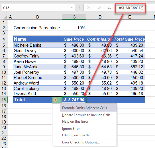
The Excel formula omits adjacent cell errors that can occur with mathematical or statistical functions, such as SUM, AVERAGE, COUNT, MIN, and MAX.
This error appears when there are cells with similar values to the one you chose that are not selected. Excel recognizes it as an error and symbolizes it with a little triangle.
I will illustrate it using the following example.
In cells A7, B7, and C7 you have the SUM function, summing cells in each column. Notice, that in the B and C columns, not all similar values are selected. In the A column, you also don’t have all cells selected (A1). But this is not the number type, so Excel understands it.
How to get rid of this error?
There are a few ways to make this error disappear.
- Change formulas to have B5 and C2 cells included.
- Remove values from cells B5 and C2.
- Click the ignore error option. You have to do it for each formula.
Getting rid of this error permanently
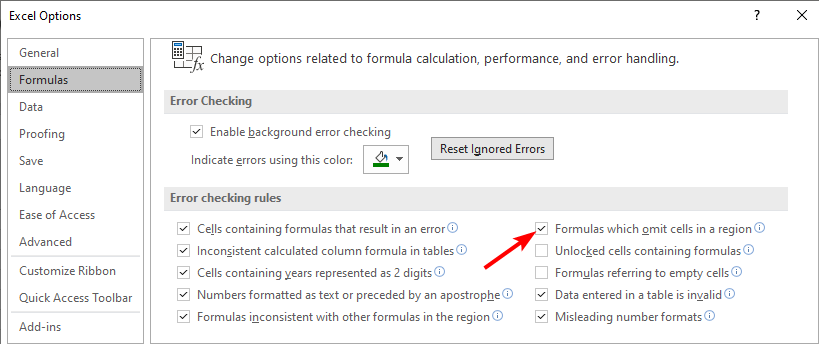
So far this error will appear until we tweak or work or click each example to ignore this error. But if you want to do this permanently and you don’t want Excel to inform you about this type of error, you can change it inside the options.
To do it, go to File >> Options >> Formulas.
On the right side, under Error checking rules uncheck the field called Formulas which omit cells in a region.
After you make this change, Excel will stop irritating you with this error message.
Post Views: 39,679
How to Fix “Formula Omits Adjacent Cells” Excel Error (2023)
The ‘Formula Omits Adjacent Cells’ is Excel’s way of saying you better recheck your formula for any missing or extra cells 🤚
You’d often see this error while running the SUM, AVERAGE, COUNT, and other mathematical or statistical functions in Excel.
What does it mean, and how can you fix it – we will see that in the guide below 👇
So continue reading and download our free sample workbook here.
Why this error appears
What is the ‘Formula Omits Adjacent Cells’ error, and why does it occur? Let me show this to you through the example below 🙈
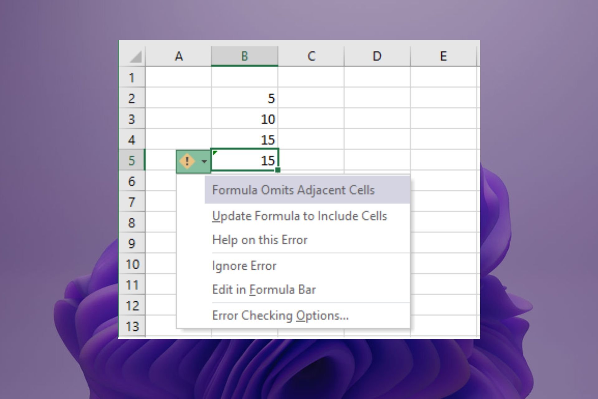
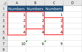
In the image below we are adding up two lists of numbers.

Each of these rows has six numbers 6️⃣
For the first list, we are summing up all the numbers.

For the second list, we are summing up only the first five numbers 5️⃣

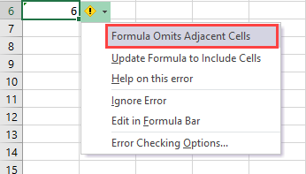
Did you see that yellow error icon and a green flag to the top left of the cell containing the sum for List 2 👀

Also, note that there’s no such sign or flag on the SUM for List 1.
Hover your cursor around the yellow error icon to see which error is this.
The “Formula omits adjacent cells” error 💀

What causes this error? When apparently, everything seems fine 🤔
This error is caused because we summed only five cells (B2:B6) for list 2.
So, we have omitted Cell B7 from the SUM formula for List 2. Whereas Cell B7 also contains a number. As all the numbers in List (A1:A7) are summed up – we have no such error there.
With that said, Excel thinks you have mistakenly left out Cell B7. That’s when Excel tells you that your formula SUM(B2:B6) omits adjacent cells (B7) 💁♀️
There are several ways how you can fix this error in Excel. We will cover them all now.
Fix #1: Change formulas to include adjacent cells
The first and easiest way to get rid of this error is to adjust your formulas:
You can change the SUM for List 2 from SUM (B2:B6) to SUM (B2:B7).

With this, technically, you have removed the error Excel thought you made 😎
So the Error signs (the green flag and yellow icon) are also removed.
Fix #2: Remove unused values
If you do not want to include Cell B7 in your calculation, remove its value from List 2.

We have only deleted the extra value causing the error (10 in Cell B7). And see, no more error signs or green flags 🚩
However, these are not some very practical ways to get rid of this error. You might not want to include B7 in your calculation. Maybe you genuinely want to sum the cells B2:B6 only.
Alternatively, you might want to retain the value in Cell B7, and deleting it might cause you to lose some data you never wanted to lose 😵
Don’t worry – here are other ways how you can remove this error in Excel without having to change your formulas or dataset.
Fix #3: Ignore the Error to remove the green triangle
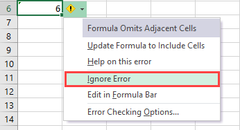
If your formulas are all set and the error has no relevance to you, you can choose to ignore it. To ignore this error and get rid of the error icons surrounding the relevant cell:
- Select the cell where the error occurs (Cell B9).
The yellow error sign will appear.
- Click on the drop-down menu icon next to this error sign.
The following list will appear 📝

- Click on Ignore Error from this list as shown above.
And the error icons will go away.

This is your way of telling Excel, “Thanks for your input, but I know my job!” 😝
If you have multiple such errors in other cells of your sheet, you’d have to ignore them for each cell showing this error.
Fix #4: Permanently remove the green triangle for this error
If you are done ticking off the error for each cell, root it out once and for all ❌
To permanently remove the green triangle caused by the ‘Formula omits Adjacent cells error’ follow these steps:
- Go to the File tab > Options.
- Under the dialog box for Excel Options, go to Formulas from the left pane.

- Under the section Error checking rules, uncheck the box for Formulas that omit cells in a region.

Excel will now no longer pose the Formula omits adjacent cells error 💪
Kasper Langmann2023-02-28T11:17:46+00:00
Page load link
I am creating a excel sheet with sum formula.
ExcelPackage pck = new ExcelPackage("D:ExcelTemplate.xlsx");
var ws = pck.Workbook.Worksheets["Sheet1"];
ws.Cells["A5"].Formula = "=SUM(A3:A4)";
but resultant A5 cell is displaying error «Formula Omits Adjacent Cells error»(It is also displaying the sum of A3 and A4 in A5 ofcourse).
When i am trying to read A5 cell i am getting «Object reference not set to an instance of an object» error.
string strA5 = ws.Cells["A5"].Value.ToString();
Please help to resolve this.
Thanks Advance.
asked Jun 13, 2013 at 16:35
![]()
Hakuna MatataHakuna Matata
1,3413 gold badges13 silver badges22 bronze badges
As far as I know, EPPlus doesn’t have a calculation engine. This means cell A5 doesn’t actually contain the calculated formula result value for «=SUM(A3:A4)». And judging from your code, I suspect A5 didn’t exist with a value, only a formula part. (Yes there are 2 parts for each cell: a formula part and a value part). So something like this:
ws.Cells["A5"].Value.ToString();
will fail with your «Object reference not set to an instance of an object.» error.
answered Jun 14, 2013 at 3:26
![]()
Vincent TanVincent Tan
3,05022 silver badges21 bronze badges
1
As of EpPlus 4.0.1.1, there is a calculation engine and an extension method Calculate(this ExcelRangeBase range). Invoke it before accessing Value property:
ws.Cells["A5"].Calculate();
and ws.Cells["A5"].Value will return the expected result.
answered Dec 23, 2014 at 5:54
![]()
DeilanDeilan
4,6903 gold badges39 silver badges52 bronze badges
See all How-To Articles
This tutorial demonstrates how to get rid of the green (trace error) triangle in Excel.
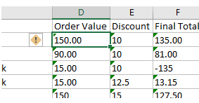
If the data contained in a cell has an error as defined by Excel, and background error checking is switched on, then a small green triangle is displayed in the top-left corner of a cell. If you click in the cell, you get a list of suggested fixes. On some occasions, you may not want to change the data in your cell, but just to hide the green triangle and ignore the error.
Switch Off Background Error Checking
To stop the green triangle error from showing, you can switch off background error checking in Excel.
- In the Ribbon, go to File > Options > Formulas > Error Checking.
- Remove the tick from the Enable background error checking option, and then click OK.
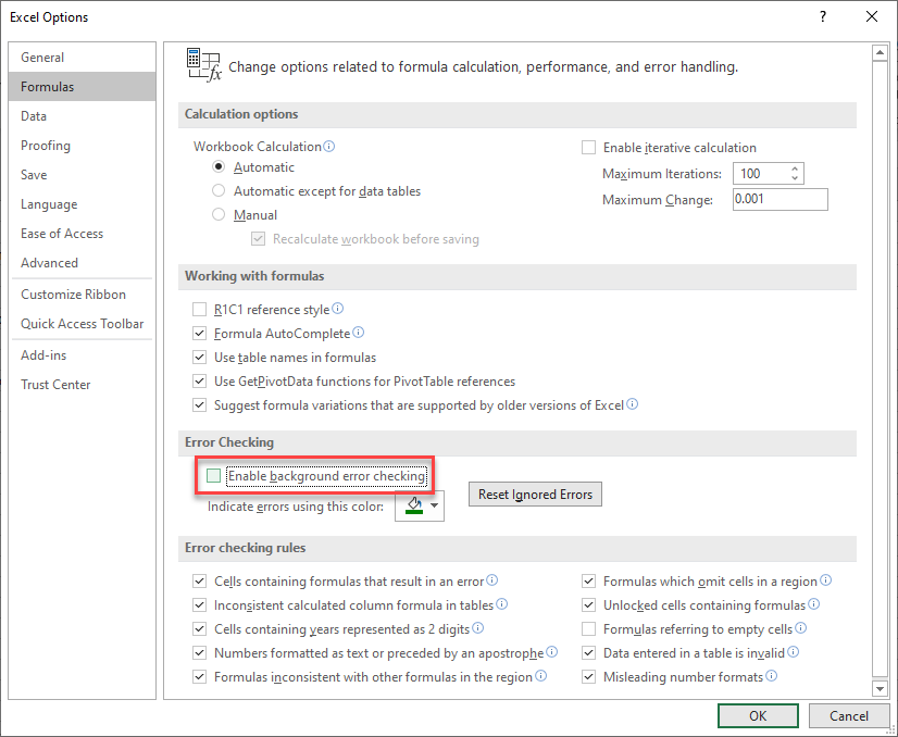
Note: This removes background error checking for the active workbook and any workbooks opened in the future.
Error Checking Rules
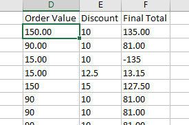
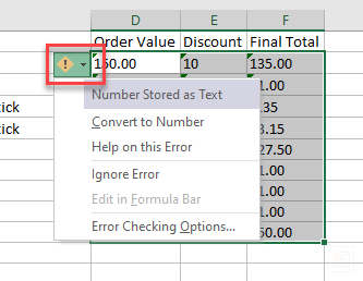
Instead of turning background error checking completely off, you can switch off individual rules that are switched on by default in Excel. For example, in the data above, the numbers are formatted as text and therefore cannot be used in calculation formulas. The green triangle alerts to this and provides a list of possible solutions. You can switch off this specific error check.
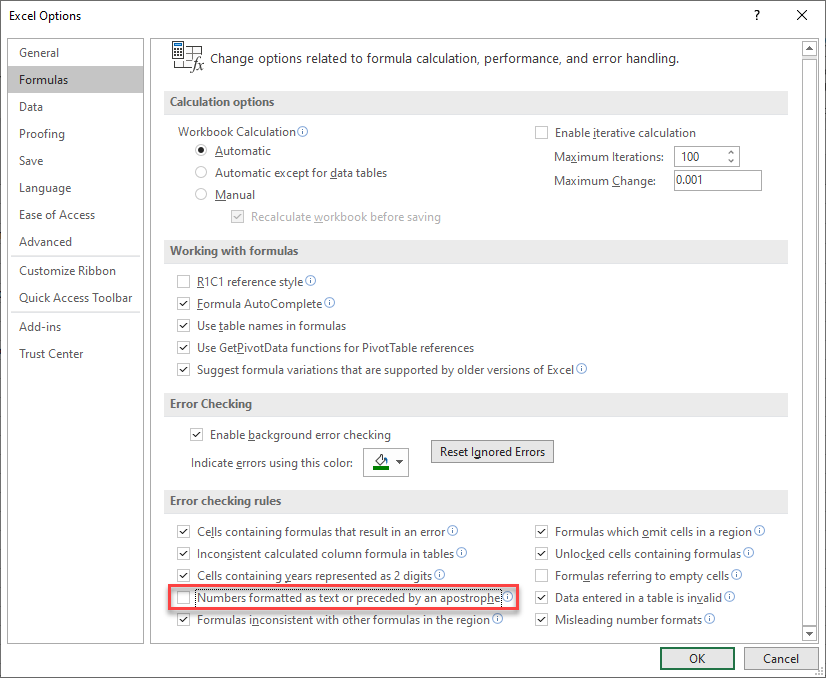
- In the Ribbon, select File > Options > Formulas > Error Checking.
- In the Error checking rules section, remove the check mark from Numbers formatted as text or preceded by an apostrophe to stop Excel from checking for this specific error, and then click OK.
Ignore Error
It’s generally best to keep the background error checking switched on, as it is very useful in showing you if you have an error in the data or in a formula.
- To remove the green triangles from cells where you are aware of the error – but do not want to see the triangle – select the cells, and then click on the little yellow exclamation mark icon.
- Click Ignore Error to remove the green triangles, or if you want to solve the error, click Convert to Number, making the cell values suitable for use in calculations.
Use the Trace Error Drop Down
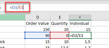
If your error has a different reason, for example a divide by zero formula error, then a different set of options is shown.
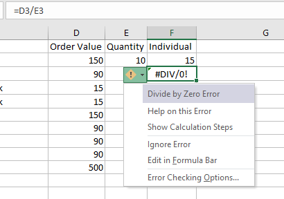
You can also ignore the error, or you can click Show Calculation Steps to resolve the error. If you click Edit in Formula Bar, Excel puts the formula into editing mode and place your mouse pointer in the formula bar so you can make changes to the formula.
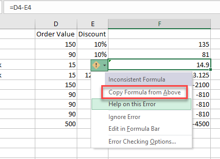
Another reason for the error could be an inconsistent formula. This occurs when the formula in the cell is different to the formula that is in the cell above. If this is the case, a different set of options appears.
To solve this problem and remove the green triangle, you can click Copy Formula from Above or, if you do not want to change the formula, you can, once again, click Ignore Error.
Common Errors in Excel
A few more common Excel errors can cause the green triangle to show in a cell – all of which can be removed using the Ignore Error option, or can be solved using Excel’s error checking options.
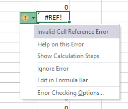
Cell Reference Error
#REF – this error normally occurs when a formula is referring to a range that is cannot find – or if rows/columns have been removed.
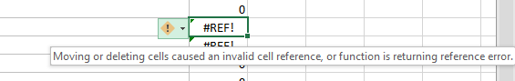
Resting your mouse on the exclamation mark icon shows you the reason for error, while clicking on the drop down shows you a list of possible solutions.
Value Error
#VALUE – this error normally occurs when you are trying to include a cell that has text in it, in a calculation.
Adjacent Cells Error
Formula Omits Adjacent Cells – this error normally occurs when you have a function like the SUM Function and are not including all the possible cells in the calculation.