Что показывает стандартная ошибка оценки

Что такое стандартная ошибка оценки? (Определение и пример)

17 авг. 2022 г.
читать 3 мин

Стандартная ошибка оценки — это способ измерения точности прогнозов, сделанных регрессионной моделью.

Часто обозначаемый σ est , он рассчитывается как:

σ est = √ Σ(y – ŷ) 2 /n

куда:

y: наблюдаемое значение
ŷ: Прогнозируемое значение
n: общее количество наблюдений

Стандартная ошибка оценки дает нам представление о том, насколько хорошо регрессионная модель соответствует набору данных. Особенно:

Чем меньше значение, тем лучше соответствие.
Чем больше значение, тем хуже соответствие.

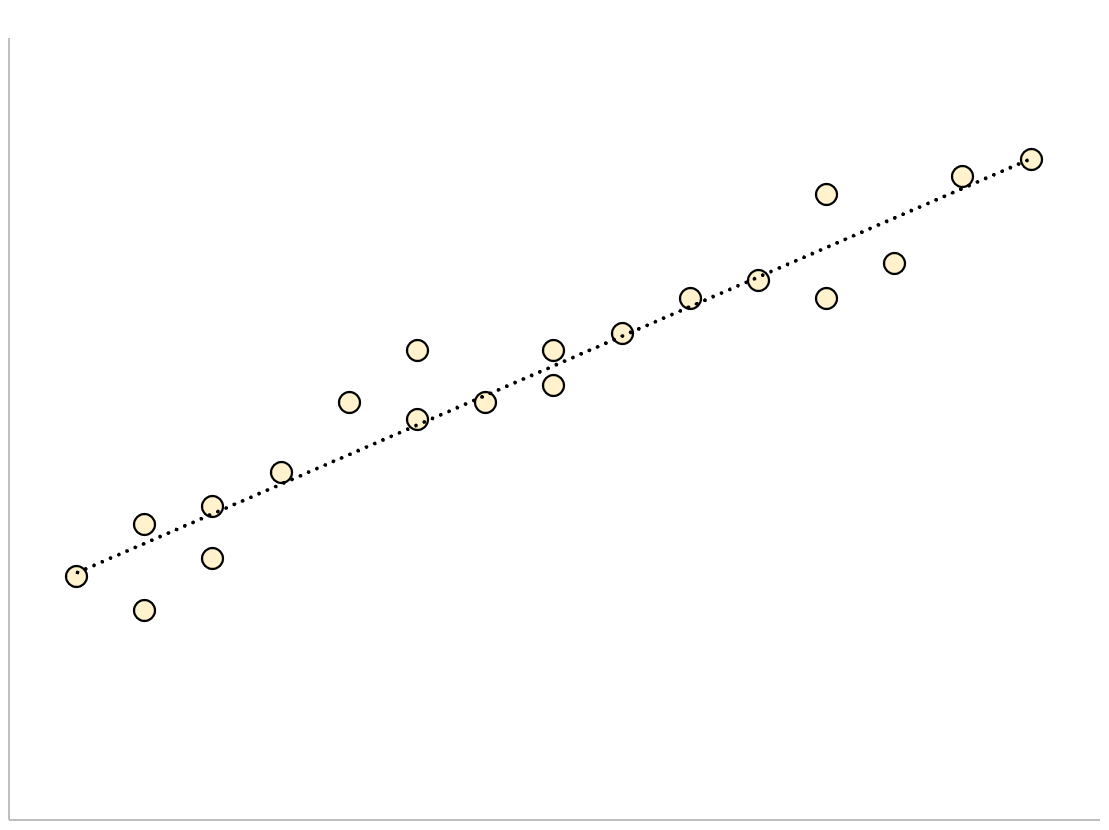
Для регрессионной модели с небольшой стандартной ошибкой оценки точки данных будут плотно сгруппированы вокруг предполагаемой линии регрессии:

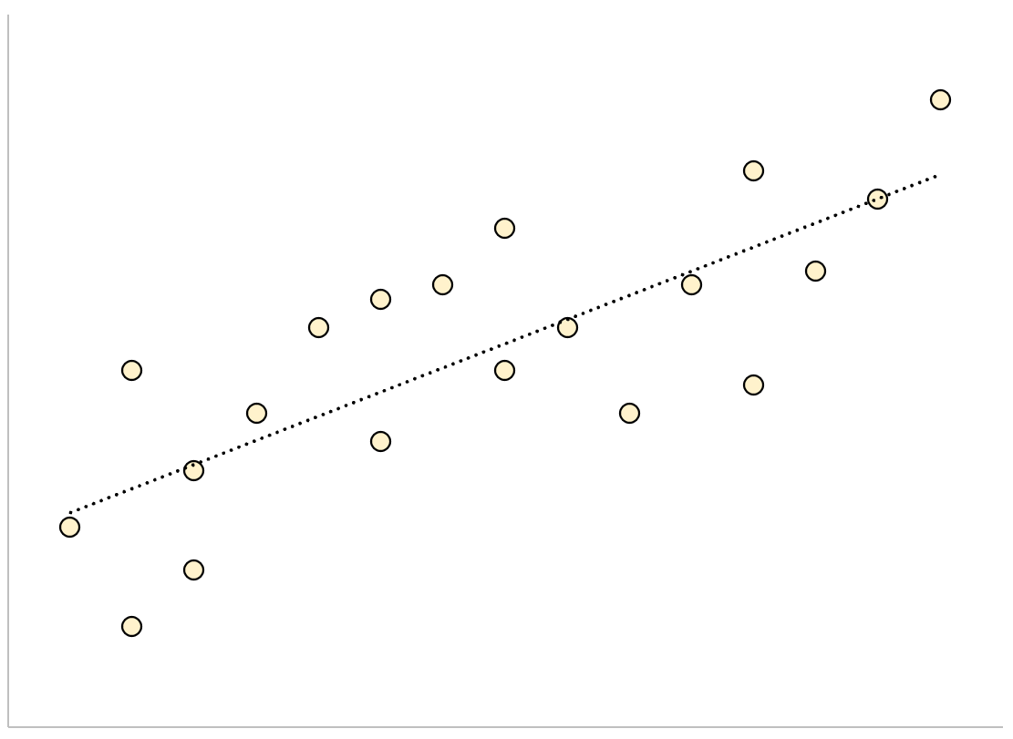
И наоборот, для регрессионной модели с большой стандартной ошибкой оценки точки данных будут более свободно разбросаны по линии регрессии:

В следующем примере показано, как рассчитать и интерпретировать стандартную ошибку оценки для регрессионной модели в Excel.

Пример: стандартная ошибка оценки в Excel

Используйте следующие шаги, чтобы вычислить стандартную ошибку оценки для регрессионной модели в Excel.

Шаг 1: введите данные

Сначала введите значения для набора данных:

Шаг 2: выполните линейную регрессию

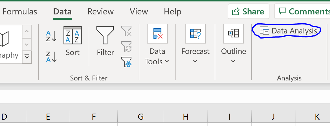
Затем щелкните вкладку « Данные » на верхней ленте. Затем выберите параметр « Анализ данных» в группе « Анализ ».

Если вы не видите эту опцию, вам нужно сначала загрузить пакет инструментов анализа .

В появившемся новом окне нажмите « Регрессия », а затем нажмите « ОК ».

В появившемся новом окне заполните следующую информацию:

Как только вы нажмете OK , появится вывод регрессии:

Мы можем использовать коэффициенты из таблицы регрессии для построения оценочного уравнения регрессии:

ŷ = 13,367 + 1,693 (х)

И мы видим, что стандартная ошибка оценки для этой регрессионной модели оказывается равной 6,006.Проще говоря, это говорит нам о том, что средняя точка данных отклоняется от линии регрессии на 6,006 единицы.

Мы можем использовать оценочное уравнение регрессии и стандартную ошибку оценки, чтобы построить 95% доверительный интервал для прогнозируемого значения определенной точки данных.

Например, предположим, что x равно 10. Используя оценочное уравнение регрессии, мы можем предсказать, что y будет равно:

ŷ = 13,367 + 1,693 * (10) = 30,297

И мы можем получить 95% доверительный интервал для этой оценки, используя следующую формулу:

95% ДИ = [ŷ – 1,96*σ расч ., ŷ + 1,96*σ расч .]

Для нашего примера доверительный интервал 95% будет рассчитываться как:

95% ДИ = [ŷ – 1,96*σ расч ., ŷ + 1,96*σ расч .]
95% ДИ = [30,297 – 1,96*6,006, 30,297 + 1,96*6,006]
95% ДИ = [18,525, 42,069]

Дополнительные ресурсы

Как выполнить простую линейную регрессию в Excel
Как выполнить множественную линейную регрессию в Excel
Как создать остаточный график в Excel

Источник

Имея
прямую регрессии, необходимо оценить
насколько сильно точки исходных данных
отклоняются от прямой регрессии. Можно
выполнить оценку разброса, аналогичную
стандартному отклонению выборки. Этот
показатель, называемый стандартной
ошибкой оценки, демонстрирует величину
отклонения точек исходных данных от
прямой регрессии в направлении оси Y.
Стандартная ошибка оценки ()
вычисляется по следующей формуле.

Стандартная
ошибка оценки измеряет степень отличия
реальных значений Y от оцененной величины.
Для сравнительно больших выборок следует
ожидать, что около 67% разностей по модулю
не будет превышать

и около 95% модулей разностей будет не
больше 2.

Стандартная
ошибка оценки подобна стандартному
отклонению. Ее можно использовать для
оценки стандартного отклонения
совокупности. Фактически

оценивает стандартное отклонение

слагаемого ошибки

в статистической модели простой линейной
регрессии. Другими словами,

оценивает общее стандартное отклонение

нормального распределения значений Y,
имеющих математические ожидания

для каждого X.

Малая
стандартная ошибка оценки, полученная
при регрессионном анализе, свидетельствует,
что все точки данных находятся очень
близко к прямой регрессии. Если стандартная
ошибка оценки велика, точки данных могут
значительно удаляться от прямой.

2.3 Прогнозирование величины y

Регрессионную
прямую можно использовать для оценки
величины переменной Y
при данных значениях переменной X. Чтобы
получить точечный прогноз, или предсказание
для данного значения X, просто вычисляется
значение найденной функции регрессии
в точке X.

Конечно
реальные значения величины Y,
соответствующие рассматриваемым
значениям величины X, к сожалению, не
лежат в точности на регрессионной
прямой. Фактически они разбросаны
относительно прямой в соответствии с
величиной
.
Более того, выборочная регрессионная
прямая является оценкой регрессионной
прямой генеральной совокупности,
основанной на выборке из определенных
пар данных. Другая случайная выборка
даст иную выборочную прямую регрессии;
это аналогично ситуации, когда различные
выборки из одной и той же генеральной
совокупности дают различные значения
выборочного среднего.

Есть
два источника неопределенности в
точечном прогнозе, использующем уравнение
регрессии.

Неопределенность,
обусловленная отклонением точек данных
от выборочной прямой регрессии.
Неопределенность,
обусловленная отклонением выборочной
прямой регрессии от регрессионной
прямой генеральной совокупности.

Интервальный
прогноз значений переменной Y
можно построить так, что при этом будут
учтены оба источника неопределенности.

Стандартная
ошибка прогноза

дает меру вариативности предсказанного
значения Y
около истинной величины Y
для данного значения X.
Стандартная ошибка прогноза равна:

Стандартная
ошибка прогноза зависит от значения X,
для которого прогнозируется величина
Y.

минимально, когда
,
поскольку тогда числитель в третьем
слагаемом под корнем в уравнении будет
0. При прочих неизменных величинах
большему отличию соответствует большее
значение стандартной ошибки прогноза.

Если
статистическая модель простой линейной
регрессии соответствует действительности,
границы интервала прогноза величины Y
равны:

где

— квантиль распределения Стьюдента с
n-2 степенями свободы ().
Если выборка велика (),
этот квантиль можно заменить соответствующим
квантилем нормального распределения.
Например, для большой выборки 95%-ный
интервал прогноза задается следующими
значениями:

Завершим
раздел обзором предположений, положенных
в основу статистической модели линейной
регрессии.

Для
заданного значения X генеральная
совокупность значений Y имеет нормальное
распределение относительно регрессионной
прямой совокупности. На практике
приемлемые результаты получаются
и
тогда, когда значения Y имеют
нормальное распределение лишь
приблизительно.
Разброс
генеральной совокупности точек данных
относительно регрессионной прямой
совокупности остается постоянным всюду
вдоль этой прямой. Иными словами, при
возрастании значений X в точках данных
дисперсия генеральной совокупности
не увеличивается и не уменьшается.
Нарушение этого предположения называется
гетероскедастичностью.
Слагаемые
ошибок

независимы между собой. Это предположение
определяет случайность выборки точек
Х-Y.
Если точки данных X-Y
записывались в течение некоторого
времени, данное предположение часто
нарушается. Вместо независимых данных,
такие последовательные наблюдения
будут давать серийно коррелированные
значения.
В
генеральной совокупности существует
линейная зависимость между X и Y.
По аналогии с простой линейной регрессией
может рассматриваться и нелинейная
зависимость между X и У. Некоторые такие
случаи будут обсуждаться ниже.

Соседние файлы в предмете [НЕСОРТИРОВАННОЕ]

Что такое стандартная ошибка оценки? (Определение и пример)

17 авг. 2022 г.
читать 3 мин

Стандартная ошибка оценки — это способ измерения точности прогнозов, сделанных регрессионной моделью.

Часто обозначаемый σ est , он рассчитывается как:

σ est = √ Σ(y – ŷ) 2 /n

куда:

y: наблюдаемое значение
ŷ: Прогнозируемое значение
n: общее количество наблюдений

Чем меньше значение, тем лучше соответствие.
Чем больше значение, тем хуже соответствие.

Пример: стандартная ошибка оценки в Excel

Используйте следующие шаги, чтобы вычислить стандартную ошибку оценки для регрессионной модели в Excel.

Шаг 1: введите данные

Сначала введите значения для набора данных:

Шаг 2: выполните линейную регрессию

Если вы не видите эту опцию, вам нужно сначала загрузить пакет инструментов анализа .

В появившемся новом окне нажмите « Регрессия », а затем нажмите « ОК ».

В появившемся новом окне заполните следующую информацию:

Как только вы нажмете OK , появится вывод регрессии:

Мы можем использовать коэффициенты из таблицы регрессии для построения оценочного уравнения регрессии:

ŷ = 13,367 + 1,693 (х)

ŷ = 13,367 + 1,693 * (10) = 30,297

И мы можем получить 95% доверительный интервал для этой оценки, используя следующую формулу:

95% ДИ = [ŷ – 1,96*σ расч ., ŷ + 1,96*σ расч .]

Для нашего примера доверительный интервал 95% будет рассчитываться как:

95% ДИ = [ŷ – 1,96*σ расч ., ŷ + 1,96*σ расч .]
95% ДИ = [30,297 – 1,96*6,006, 30,297 + 1,96*6,006]
95% ДИ = [18,525, 42,069]

Дополнительные ресурсы

Загрузить PDF

Стандартная ошибка оценки служит для того, чтобы выяснить, как линия регрессии соответствует набору данных. Если у вас есть набор данных, полученных в результате измерения, эксперимента, опроса или из другого источника, создайте линию регрессии, чтобы оценить дополнительные данные. Стандартная ошибка оценки характеризует, насколько верна линия регрессии.

1

Создайте таблицу с данными. Таблица должна состоять из пяти столбцов, и призвана облегчить вашу работу с данными. Чтобы вычислить стандартную ошибку оценки, понадобятся пять величин. Поэтому разделите таблицу на пять столбцов. Обозначьте эти столбцы так:^[1]
2
Введите данные в таблицу. Когда вы проведете эксперимент или опрос, вы получите пары данных — независимую переменную обозначим как , а зависимую или конечную переменную как . Введите эти значения в первые два столбца таблицы.
- Не перепутайте данные. Помните, что определенному значению независимой переменной должно соответствовать конкретное значение зависимой переменной.
- Например, рассмотрим следующий набор пар данных:
  - (1,2)
  - (2,4)
  - (3,5)
  - (4,4)
  - (5,5)
3
Вычислите линию регрессии. Сделайте это на основе представленных данных. Эта линия также называется линией наилучшего соответствия или линией наименьших квадратов. Расчет можно сделать вручную, но это довольно утомительно. Поэтому рекомендуем воспользоваться графическим калькулятором или онлайн-сервисом, которые быстро вычислят линию регрессии по вашим данным.^[2]
- В этой статье предполагается, что уравнение линии регрессии дано (известно).
- В нашем примере линия регрессии описывается уравнением $y^{{prime }}=0,6x+2,2$ .
4

Вычислите прогнозируемые значения по линии регрессии. С помощью уравнения линии регрессии можно вычислить прогнозируемые значения «y» для значений «x», которые есть и которых нет в наборе данных.

Реклама

1
Вычислите ошибку каждого прогнозируемого значения. В четвертом столбце таблицы запишите ошибку каждого прогнозируемого значения. В частности, вычтите прогнозируемое значение ( $y^{{prime }}$ ) из фактического (наблюдаемого) значения ().^[3]
- В нашем примере вычисления будут выглядеть так:
2
Вычислите квадраты ошибок. Возведите в квадрат каждое значение четвертого столбца, а результаты запишите в последнем (пятом) столбце таблицы.
- В нашем примере вычисления будут выглядеть так:
3
Найдите сумму квадратов ошибок. Она пригодится для вычисления стандартного отклонения, дисперсии и других величин. Чтобы найти сумму квадратов ошибок, сложите все значения пятого столбца. ^[4]
- В нашем примере вычисления будут выглядеть так:
4
Завершите расчеты. Стандартная ошибка оценки — это квадратный корень из среднего значения суммы квадратов ошибок. Обычно ошибка оценки обозначается греческой буквой . Поэтому сначала разделите сумму квадратов ошибок на число пар данных. А потом из полученного значения извлеките квадратный корень.^[5]
- Если рассматриваемые данные представляют всю совокупность, среднее значение находится так: сумму нужно разделить на N (количество пар данных). Если же рассматриваемые данные представляют некоторую выборку, вместо N подставьте N-2.
- В нашем примере, скорее всего, имеет место выборка, потому что мы рассматриваем всего 5 пар данных. Поэтому стандартную ошибку оценки вычислите следующим образом:
5
Интерпретируйте полученный результат. Стандартная ошибка оценки — это статистический показатель, которые оценивает, насколько близко измеренные данные лежат к линии регрессии. Ошибка оценка «0» означает, что каждая точка лежит непосредственно на линии. Чем выше ошибка оценки, тем дальше от линии регрессии лежат точки.^[6]
- В нашем примере выборка достаточно маленькая, поэтому стандартная оценка ошибки 0,894 является довольно низкой и характеризует близко расположенные данные.
Реклама

Об этой статье

Эту страницу просматривали 4133 раза.

Была ли эта статья полезной?

Download Article

The standard error of estimate is used to determine how well a straight line can describe values of a data set. When you have a collection of data from some measurement, experiment, survey or other source, you can create a line of regression to estimate additional data. With the standard error of estimate, you get a score that describes how good the regression line is.

1

Create a five column data table. Any statistical work is generally made easier by having your data in a concise format. A simple table serves this purpose very well. To calculate the standard error of estimate, you will be using five different measurements or calculations. Therefore, creating a five-column table is helpful. Label the five columns as follows:^[1]
2
Enter the data values for your measured data. After collecting your data, you will have pairs of data values. For these statistical calculations, the independent variable is labeled and the dependent, or resulting, variable is . Enter these values into the first two columns of your data table.^[2]
- The order of the data and the pairing is important for these calculations. You need to be careful to keep your paired data points together in order.
- For the sample calculations shown above, the data pairs are as follows:
  - (1,2)
  - (2,4)
  - (3,5)
  - (4,4)
  - (5,5)
Advertisement
3
Calculate a regression line. Using your data results, you will be able to calculate a regression line. This is also called a line of best fit or the least squares line. The calculation is tedious but can be done by hand. Alternatively, you can use a handheld graphing calculator or some online programs that will quickly calculate a best fit line using your data.^[3]
- For this article, it is assumed that you will have the regression line equation available or that it has been predicted by some prior means.
- For the sample data set in the image above, the regression line is $y^{{prime }}=0.6x+2.2$ .
4

Calculate predicted values from the regression line. Using the equation of that line, you can calculate predicted y-values for each x-value in your study, or for other theoretical x-values that you did not measure.^[4]

1
Calculate the error of each predicted value. In the fourth column of your data table, you will calculate and record the error of each predicted value. Specifically, subtract the predicted value ( $y^{{prime }}$ ) from the actual observed value ().^[5]
- For the data in the sample set, these calculations are as follows:
2
Calculate the squares of the errors. Take each value in the fourth column and square it by multiplying it by itself. Fill in these results in the final column of your data table.
- For the sample data set, these calculations are as follows:
3
Find the sum of the squared errors (SSE). The statistical value known as the sum of squared errors (SSE) is a useful step in finding standard deviation, variance and other measurements. To find the SSE from your data table, add the values in the fifth column of your data table.^[6]
- For this sample data set, this calculation is as follows:
4
Finalize your calculations. The Standard Error of the Estimate is the square root of the average of the SSE. It is generally represented with the Greek letter . Therefore, the first calculation is to divide the SSE score by the number of measured data points. Then, find the square root of that result.^[7]
- If the measured data represents an entire population, then you will find the average by dividing by N, the number of data points. However, if you are working with a smaller sample set of the population, then substitute N-2 in the denominator.
- For the sample data set in this article, we can assume that it is a sample set and not a population, just because there are only 5 data values. Therefore, calculate the Standard Error of the Estimate as follows:
5
Interpret your result. The Standard Error of the Estimate is a statistical figure that tells you how well your measured data relates to a theoretical straight line, the line of regression. A score of 0 would mean a perfect match, that every measured data point fell directly on the line. Widely scattered data will have a much higher score.^[8]
- With this small sample set, the standard error score of 0.894 is quite low and represents well organized data results.

Ask a Question

200 characters left

Include your email address to get a message when this question is answered.

Submit

Video

Thanks for submitting a tip for review!

References

About This Article

Article SummaryX

To calculate the standard error of estimate, create a five-column data table. In the first two columns, enter the values for your measured data, and enter the values from the regression line in the third column. In the fourth column, calculate the predicted values from the regression line using the equation from that line. These are the errors. Fill in the fifth column by multiplying each error by itself. Add together all of the values in column 5, then take the square root of that number to get the standard error of estimate. To learn how to organize the data pairs, keep reading!

Did this summary help you?

Thanks to all authors for creating a page that has been read 186,173 times.

Did this article help you?

Download Article

1

Create a five column data table. Any statistical work is generally made easier by having your data in a concise format. A simple table serves this purpose very well. To calculate the standard error of estimate, you will be using five different measurements or calculations. Therefore, creating a five-column table is helpful. Label the five columns as follows:^[1]
2
Enter the data values for your measured data. After collecting your data, you will have pairs of data values. For these statistical calculations, the independent variable is labeled and the dependent, or resulting, variable is . Enter these values into the first two columns of your data table.^[2]
- The order of the data and the pairing is important for these calculations. You need to be careful to keep your paired data points together in order.
- For the sample calculations shown above, the data pairs are as follows:
  - (1,2)
  - (2,4)
  - (3,5)
  - (4,4)
  - (5,5)
Advertisement
3
Calculate a regression line. Using your data results, you will be able to calculate a regression line. This is also called a line of best fit or the least squares line. The calculation is tedious but can be done by hand. Alternatively, you can use a handheld graphing calculator or some online programs that will quickly calculate a best fit line using your data.^[3]
- For this article, it is assumed that you will have the regression line equation available or that it has been predicted by some prior means.
- For the sample data set in the image above, the regression line is $y^{{prime }}=0.6x+2.2$ .
4

Calculate predicted values from the regression line. Using the equation of that line, you can calculate predicted y-values for each x-value in your study, or for other theoretical x-values that you did not measure.^[4]

1
Calculate the error of each predicted value. In the fourth column of your data table, you will calculate and record the error of each predicted value. Specifically, subtract the predicted value ( $y^{{prime }}$ ) from the actual observed value ().^[5]
- For the data in the sample set, these calculations are as follows:
2
Calculate the squares of the errors. Take each value in the fourth column and square it by multiplying it by itself. Fill in these results in the final column of your data table.
- For the sample data set, these calculations are as follows:
3
Find the sum of the squared errors (SSE). The statistical value known as the sum of squared errors (SSE) is a useful step in finding standard deviation, variance and other measurements. To find the SSE from your data table, add the values in the fifth column of your data table.^[6]
- For this sample data set, this calculation is as follows:
4
Finalize your calculations. The Standard Error of the Estimate is the square root of the average of the SSE. It is generally represented with the Greek letter . Therefore, the first calculation is to divide the SSE score by the number of measured data points. Then, find the square root of that result.^[7]
- If the measured data represents an entire population, then you will find the average by dividing by N, the number of data points. However, if you are working with a smaller sample set of the population, then substitute N-2 in the denominator.
- For the sample data set in this article, we can assume that it is a sample set and not a population, just because there are only 5 data values. Therefore, calculate the Standard Error of the Estimate as follows:
5
Interpret your result. The Standard Error of the Estimate is a statistical figure that tells you how well your measured data relates to a theoretical straight line, the line of regression. A score of 0 would mean a perfect match, that every measured data point fell directly on the line. Widely scattered data will have a much higher score.^[8]
- With this small sample set, the standard error score of 0.894 is quite low and represents well organized data results.

Ask a Question

200 characters left

Include your email address to get a message when this question is answered.

Submit

Video

Thanks for submitting a tip for review!

References

About This Article

Article SummaryX

Did this summary help you?

Thanks to all authors for creating a page that has been read 186,173 times.

Did this article help you?

Источник

2.3 Прогнозирование величины y

Есть
два источника неопределенности в
точечном прогнозе, использующем уравнение
регрессии.

Неопределенность,
обусловленная отклонением точек данных
от выборочной прямой регрессии.
Неопределенность,
обусловленная отклонением выборочной
прямой регрессии от регрессионной
прямой генеральной совокупности.

Завершим
раздел обзором предположений, положенных
в основу статистической модели линейной
регрессии.

Для
заданного значения X генеральная
совокупность значений Y имеет нормальное
распределение относительно регрессионной
прямой совокупности. На практике
приемлемые результаты получаются
и
тогда, когда значения Y имеют
нормальное распределение лишь
приблизительно.
Разброс
генеральной совокупности точек данных
относительно регрессионной прямой
совокупности остается постоянным всюду
вдоль этой прямой. Иными словами, при
возрастании значений X в точках данных
дисперсия генеральной совокупности
не увеличивается и не уменьшается.
Нарушение этого предположения называется
гетероскедастичностью.
Слагаемые
ошибок

независимы между собой. Это предположение
определяет случайность выборки точек
Х-Y.
Если точки данных X-Y
записывались в течение некоторого
времени, данное предположение часто
нарушается. Вместо независимых данных,
такие последовательные наблюдения
будут давать серийно коррелированные
значения.
В
генеральной совокупности существует
линейная зависимость между X и Y.
По аналогии с простой линейной регрессией
может рассматриваться и нелинейная
зависимость между X и У. Некоторые такие
случаи будут обсуждаться ниже.

Соседние файлы в предмете [НЕСОРТИРОВАННОЕ]

Источник

From Wikipedia, the free encyclopedia

For a value that is sampled with an unbiased normally distributed error, the above depicts the proportion of samples that would fall between 0, 1, 2, and 3 standard deviations above and below the actual value.

The standard error (SE)^[1] of a statistic (usually an estimate of a parameter) is the standard deviation of its sampling distribution^[2] or an estimate of that standard deviation. If the statistic is the sample mean, it is called the standard error of the mean (SEM).^[1]

The sampling distribution of a mean is generated by repeated sampling from the same population and recording of the sample means obtained. This forms a distribution of different means, and this distribution has its own mean and variance. Mathematically, the variance of the sampling mean distribution obtained is equal to the variance of the population divided by the sample size. This is because as the sample size increases, sample means cluster more closely around the population mean.

Therefore, the relationship between the standard error of the mean and the standard deviation is such that, for a given sample size, the standard error of the mean equals the standard deviation divided by the square root of the sample size.^[1] In other words, the standard error of the mean is a measure of the dispersion of sample means around the population mean.

In regression analysis, the term «standard error» refers either to the square root of the reduced chi-squared statistic or the standard error for a particular regression coefficient (as used in, say, confidence intervals).

Standard error of the sample mean[edit]

Exact value[edit]

Suppose a statistically independent sample of observations ${displaystyle x_{1},x_{2},ldots ,x_{n}}$ is taken from a statistical population with a standard deviation of sigma . The mean value calculated from the sample, , will have an associated standard error on the mean, ${displaystyle {sigma }_{bar {x}}}$ , given by:^[1]

${displaystyle {sigma }_{bar {x}} ={frac {sigma }{sqrt {n}}}}$ .

Practically this tells us that when trying to estimate the value of a population mean, due to the factor , reducing the error on the estimate by a factor of two requires acquiring four times as many observations in the sample; reducing it by a factor of ten requires a hundred times as many observations.

Estimate[edit]

The standard deviation sigma of the population being sampled is seldom known. Therefore, the standard error of the mean is usually estimated by replacing sigma with the sample standard deviation $sigma _{x}$ instead:

${displaystyle {sigma }_{bar {x}} approx {frac {sigma _{x}}{sqrt {n}}}}$

As this is only an estimator for the true «standard error», it is common to see other notations here such as:

${displaystyle {widehat {sigma }}_{bar {x}}approx {frac {sigma _{x}}{sqrt {n}}}}$

or alternately ${displaystyle {s}_{bar {x}} approx {frac {s}{sqrt {n}}}}$ .

A common source of confusion occurs when failing to distinguish clearly between:

Accuracy of the estimator[edit]

When the sample size is small, using the standard deviation of the sample instead of the true standard deviation of the population will tend to systematically underestimate the population standard deviation, and therefore also the standard error. With n = 2, the underestimate is about 25%, but for n = 6, the underestimate is only 5%. Gurland and Tripathi (1971) provide a correction and equation for this effect.^[3] Sokal and Rohlf (1981) give an equation of the correction factor for small samples of n < 20.^[4] See unbiased estimation of standard deviation for further discussion.

Derivation[edit]

The standard error on the mean may be derived from the variance of a sum of independent random variables,^[5] given the definition of variance and some simple properties thereof. If ${displaystyle x_{1},x_{2},ldots ,x_{n}}$ is a sample of independent observations from a population with mean and standard deviation sigma , then we can define the total

${displaystyle T=(x_{1}+x_{2}+cdots +x_{n})}$

which due to the Bienaymé formula, will have variance

${displaystyle operatorname {Var} (T)approx {big (}operatorname {Var} (x_{1})+operatorname {Var} (x_{2})+cdots +operatorname {Var} (x_{n}){big )}=nsigma ^{2}.}$

where we’ve approximated the standard deviations, i.e., the uncertainties, of the measurements themselves with the best value for the standard deviation of the population. The mean of these measurements is simply given by

The variance of the mean is then

${displaystyle operatorname {Var} ({bar {x}})=operatorname {Var} left({frac {T}{n}}right)={frac {1}{n^{2}}}operatorname {Var} (T)={frac {1}{n^{2}}}nsigma ^{2}={frac {sigma ^{2}}{n}}.}$

The standard error is, by definition, the standard deviation of which is simply the square root of the variance:

${displaystyle sigma _{bar {x}}={sqrt {frac {sigma ^{2}}{n}}}={frac {sigma }{sqrt {n}}}}$

For correlated random variables the sample variance needs to be computed according to the Markov chain central limit theorem.

Independent and identically distributed random variables with random sample size[edit]

There are cases when a sample is taken without knowing, in advance, how many observations will be acceptable according to some criterion. In such cases, the sample size is a random variable whose variation adds to the variation of such that,

${displaystyle operatorname {Var} (T)=operatorname {E} (N)operatorname {Var} (X)+operatorname {Var} (N){big (}operatorname {E} (X){big )}^{2}}$

^[6]

If has a Poisson distribution, then with estimator . Hence the estimator of becomes ${displaystyle nS_{X}^{2}+n{bar {X}}^{2}}$ , leading the following formula for standard error:

${displaystyle operatorname {Standard~Error} ({bar {X}})={sqrt {frac {S_{X}^{2}+{bar {X}}^{2}}{n}}}}$

(since the standard deviation is the square root of the variance)

Student approximation when σ value is unknown[edit]

In many practical applications, the true value of σ is unknown. As a result, we need to use a distribution that takes into account that spread of possible σ’s.
When the true underlying distribution is known to be Gaussian, although with unknown σ, then the resulting estimated distribution follows the Student t-distribution. The standard error is the standard deviation of the Student t-distribution. T-distributions are slightly different from Gaussian, and vary depending on the size of the sample. Small samples are somewhat more likely to underestimate the population standard deviation and have a mean that differs from the true population mean, and the Student t-distribution accounts for the probability of these events with somewhat heavier tails compared to a Gaussian. To estimate the standard error of a Student t-distribution it is sufficient to use the sample standard deviation «s» instead of σ, and we could use this value to calculate confidence intervals.

Note: The Student’s probability distribution is approximated well by the Gaussian distribution when the sample size is over 100. For such samples one can use the latter distribution, which is much simpler.

Assumptions and usage[edit]

An example of how is used is to make confidence intervals of the unknown population mean. If the sampling distribution is normally distributed, the sample mean, the standard error, and the quantiles of the normal distribution can be used to calculate confidence intervals for the true population mean. The following expressions can be used to calculate the upper and lower 95% confidence limits, where is equal to the sample mean, is equal to the standard error for the sample mean, and 1.96 is the approximate value of the 97.5 percentile point of the normal distribution:

Upper 95% limit

{displaystyle ={bar {x}}+(operatorname {SE} times 1.96),}

and

Lower 95% limit

In particular, the standard error of a sample statistic (such as sample mean) is the actual or estimated standard deviation of the sample mean in the process by which it was generated. In other words, it is the actual or estimated standard deviation of the sampling distribution of the sample statistic. The notation for standard error can be any one of SE, SEM (for standard error of measurement or mean), or S_E.

Standard errors provide simple measures of uncertainty in a value and are often used because:

in many cases, if the standard error of several individual quantities is known then the standard error of some function of the quantities can be easily calculated;
when the probability distribution of the value is known, it can be used to calculate an exact confidence interval;
when the probability distribution is unknown, Chebyshev’s or the Vysochanskiï–Petunin inequalities can be used to calculate a conservative confidence interval; and
as the sample size tends to infinity the central limit theorem guarantees that the sampling distribution of the mean is asymptotically normal.

Standard error of mean versus standard deviation[edit]

In scientific and technical literature, experimental data are often summarized either using the mean and standard deviation of the sample data or the mean with the standard error. This often leads to confusion about their interchangeability. However, the mean and standard deviation are descriptive statistics, whereas the standard error of the mean is descriptive of the random sampling process. The standard deviation of the sample data is a description of the variation in measurements, while the standard error of the mean is a probabilistic statement about how the sample size will provide a better bound on estimates of the population mean, in light of the central limit theorem.^[7]

Put simply, the standard error of the sample mean is an estimate of how far the sample mean is likely to be from the population mean, whereas the standard deviation of the sample is the degree to which individuals within the sample differ from the sample mean.^[8] If the population standard deviation is finite, the standard error of the mean of the sample will tend to zero with increasing sample size, because the estimate of the population mean will improve, while the standard deviation of the sample will tend to approximate the population standard deviation as the sample size increases.

Extensions[edit]

Finite population correction (FPC)[edit]

The formula given above for the standard error assumes that the population is infinite. Nonetheless, it is often used for finite populations when people are interested in measuring the process that created the existing finite population (this is called an analytic study). Though the above formula is not exactly correct when the population is finite, the difference between the finite- and infinite-population versions will be small when sampling fraction is small (e.g. a small proportion of a finite population is studied). In this case people often do not correct for the finite population, essentially treating it as an «approximately infinite» population.

If one is interested in measuring an existing finite population that will not change over time, then it is necessary to adjust for the population size (called an enumerative study). When the sampling fraction (often termed f) is large (approximately at 5% or more) in an enumerative study, the estimate of the standard error must be corrected by multiplying by a »finite population correction» (a.k.a.: FPC):^[9]
^[10]

${displaystyle operatorname {FPC} ={sqrt {frac {N-n}{N-1}}}}$

which, for large N:

${displaystyle operatorname {FPC} approx {sqrt {1-{frac {n}{N}}}}={sqrt {1-f}}}$

to account for the added precision gained by sampling close to a larger percentage of the population. The effect of the FPC is that the error becomes zero when the sample size n is equal to the population size N.

This happens in survey methodology when sampling without replacement. If sampling with replacement, then FPC does not come into play.

Correction for correlation in the sample[edit]

Expected error in the mean of A for a sample of n data points with sample bias coefficient ρ. The unbiased standard error plots as the ρ = 0 diagonal line with log-log slope −½.

If values of the measured quantity A are not statistically independent but have been obtained from known locations in parameter space x, an unbiased estimate of the true standard error of the mean (actually a correction on the standard deviation part) may be obtained by multiplying the calculated standard error of the sample by the factor f:

$f={sqrt {frac {1+rho }{1-rho }}},$

where the sample bias coefficient ρ is the widely used Prais–Winsten estimate of the autocorrelation-coefficient (a quantity between −1 and +1) for all sample point pairs. This approximate formula is for moderate to large sample sizes; the reference gives the exact formulas for any sample size, and can be applied to heavily autocorrelated time series like Wall Street stock quotes. Moreover, this formula works for positive and negative ρ alike.^[11] See also unbiased estimation of standard deviation for more discussion.

References[edit]

^ ^a ^b ^c ^d Altman, Douglas G; Bland, J Martin (2005-10-15). «Standard deviations and standard errors». BMJ: British Medical Journal. 331 (7521): 903. doi:10.1136/bmj.331.7521.903. ISSN 0959-8138. PMC 1255808. PMID 16223828.
^ Everitt, B. S. (2003). The Cambridge Dictionary of Statistics. CUP. ISBN 978-0-521-81099-9.
^ Gurland, J; Tripathi RC (1971). «A simple approximation for unbiased estimation of the standard deviation». American Statistician. 25 (4): 30–32. doi:10.2307/2682923. JSTOR 2682923.
^ Sokal; Rohlf (1981). Biometry: Principles and Practice of Statistics in Biological Research (2nd ed.). p. 53. ISBN 978-0-7167-1254-1.
^ Hutchinson, T. P. (1993). Essentials of Statistical Methods, in 41 pages. Adelaide: Rumsby. ISBN 978-0-646-12621-0.
^ Cornell, J R, and Benjamin, C A, Probability, Statistics, and Decisions for Civil Engineers, McGraw-Hill, NY, 1970, ISBN 0486796094, pp. 178–9.
^ Barde, M. (2012). «What to use to express the variability of data: Standard deviation or standard error of mean?». Perspect. Clin. Res. 3 (3): 113–116. doi:10.4103/2229-3485.100662. PMC 3487226. PMID 23125963.
^ Wassertheil-Smoller, Sylvia (1995). Biostatistics and Epidemiology : A Primer for Health Professionals (Second ed.). New York: Springer. pp. 40–43. ISBN 0-387-94388-9.
^ Isserlis, L. (1918). «On the value of a mean as calculated from a sample». Journal of the Royal Statistical Society. 81 (1): 75–81. doi:10.2307/2340569. JSTOR 2340569. (Equation 1)
^ Bondy, Warren; Zlot, William (1976). «The Standard Error of the Mean and the Difference Between Means for Finite Populations». The American Statistician. 30 (2): 96–97. doi:10.1080/00031305.1976.10479149. JSTOR 2683803. (Equation 2)
^ Bence, James R. (1995). «Analysis of Short Time Series: Correcting for Autocorrelation». Ecology. 76 (2): 628–639. doi:10.2307/1941218. JSTOR 1941218.

Источник

Загрузить PDF

1

Создайте таблицу с данными. Таблица должна состоять из пяти столбцов, и призвана облегчить вашу работу с данными. Чтобы вычислить стандартную ошибку оценки, понадобятся пять величин. Поэтому разделите таблицу на пять столбцов. Обозначьте эти столбцы так:^[1]
2
Введите данные в таблицу. Когда вы проведете эксперимент или опрос, вы получите пары данных — независимую переменную обозначим как , а зависимую или конечную переменную как . Введите эти значения в первые два столбца таблицы.
- Не перепутайте данные. Помните, что определенному значению независимой переменной должно соответствовать конкретное значение зависимой переменной.
- Например, рассмотрим следующий набор пар данных:
  - (1,2)
  - (2,4)
  - (3,5)
  - (4,4)
  - (5,5)
3
Вычислите линию регрессии. Сделайте это на основе представленных данных. Эта линия также называется линией наилучшего соответствия или линией наименьших квадратов. Расчет можно сделать вручную, но это довольно утомительно. Поэтому рекомендуем воспользоваться графическим калькулятором или онлайн-сервисом, которые быстро вычислят линию регрессии по вашим данным.^[2]
- В этой статье предполагается, что уравнение линии регрессии дано (известно).
- В нашем примере линия регрессии описывается уравнением $y^{{prime }}=0,6x+2,2$ .
4

Вычислите прогнозируемые значения по линии регрессии. С помощью уравнения линии регрессии можно вычислить прогнозируемые значения «y» для значений «x», которые есть и которых нет в наборе данных.

Реклама

1
Вычислите ошибку каждого прогнозируемого значения. В четвертом столбце таблицы запишите ошибку каждого прогнозируемого значения. В частности, вычтите прогнозируемое значение ( $y^{{prime }}$ ) из фактического (наблюдаемого) значения ().^[3]
- В нашем примере вычисления будут выглядеть так:
2
Вычислите квадраты ошибок. Возведите в квадрат каждое значение четвертого столбца, а результаты запишите в последнем (пятом) столбце таблицы.
- В нашем примере вычисления будут выглядеть так:
3
Найдите сумму квадратов ошибок. Она пригодится для вычисления стандартного отклонения, дисперсии и других величин. Чтобы найти сумму квадратов ошибок, сложите все значения пятого столбца. ^[4]
- В нашем примере вычисления будут выглядеть так:
4
Завершите расчеты. Стандартная ошибка оценки — это квадратный корень из среднего значения суммы квадратов ошибок. Обычно ошибка оценки обозначается греческой буквой . Поэтому сначала разделите сумму квадратов ошибок на число пар данных. А потом из полученного значения извлеките квадратный корень.^[5]
- Если рассматриваемые данные представляют всю совокупность, среднее значение находится так: сумму нужно разделить на N (количество пар данных). Если же рассматриваемые данные представляют некоторую выборку, вместо N подставьте N-2.
- В нашем примере, скорее всего, имеет место выборка, потому что мы рассматриваем всего 5 пар данных. Поэтому стандартную ошибку оценки вычислите следующим образом:
5
Интерпретируйте полученный результат. Стандартная ошибка оценки — это статистический показатель, которые оценивает, насколько близко измеренные данные лежат к линии регрессии. Ошибка оценка «0» означает, что каждая точка лежит непосредственно на линии. Чем выше ошибка оценки, тем дальше от линии регрессии лежат точки.^[6]
- В нашем примере выборка достаточно маленькая, поэтому стандартная оценка ошибки 0,894 является довольно низкой и характеризует близко расположенные данные.
Реклама

Об этой статье

Эту страницу просматривали 4741 раз.

Была ли эта статья полезной?

Источник

Что такое стандартная ошибка оценки? (Определение и пример)

Пример: стандартная ошибка оценки в Excel

Дополнительные ресурсы

2.3 Прогнозирование величины y

Что такое стандартная ошибка оценки? (Определение и пример)

Пример: стандартная ошибка оценки в Excel

Дополнительные ресурсы

Об этой статье

Была ли эта статья полезной?

Video

References

About This Article

Did this article help you?

Video

References

About This Article

Did this article help you?

2.3 Прогнозирование величины y

Standard error of the sample mean[edit]

Exact value[edit]

Estimate[edit]

Accuracy of the estimator[edit]

Derivation[edit]

Independent and identically distributed random variables with random sample size[edit]

Student approximation when σ value is unknown[edit]

Assumptions and usage[edit]

Standard error of mean versus standard deviation[edit]

Extensions[edit]

Finite population correction (FPC)[edit]

Correction for correlation in the sample[edit]

See also[edit]

References[edit]

Об этой статье

Была ли эта статья полезной?

Возможно, вам также будет интересно: